16.1 Population Genetics
Elizabeth Dahlhoff
Learning Objectives
By the end of this section, you will be able to do the following:
- Define population genetics and describe how it is used in the study of mechanisms of evolution and adaptation.
- Define the Hardy-Weinberg principle and discuss its importance.
- Understand biological processes that cause populations to deviate from the Hardy-Weinberg equilibrium.
- Understand how to calculate allele and genotype frequencies for populations that conform to assumptions of Hardy-Weinberg.
The Modern Synthesis of Genetics and Evolution
As mentioned at the beginning of the previous chapter, mechanisms of inheritance, or genetics, were not understood at the time Charles Darwin and Alfred Russel Wallace were developing their idea of natural selection. This lack of understanding was a stumbling block to understanding many aspects of evolution. In fact, the predominant (and incorrect) genetic theory of the time, blending inheritance, made it difficult to understand how natural selection might operate. Darwin and Wallace were unaware of the genetics work by Austrian monk Gregor Mendel, which was published in 1866, not long after publication of Darwin’s book, On the Origin of Species. Mendel’s work was rediscovered in the early twentieth century at which time geneticists were rapidly coming to an understanding of the basics of inheritance. Initially, the newly discovered particulate nature of genes made it difficult for biologists to understand how gradual evolution could occur. But over the next few decades genetics and evolution were integrated in what became known as the modern synthesis—the coherent understanding of the relationship between natural selection and genetics that took shape by the 1940s and is generally accepted today. In sum, the modern synthesis describes how evolutionary processes, such as natural selection, can affect a population’s genetic makeup, and, in turn, how this can result in the gradual evolution of populations and species.
Population Genetics
Recall that a gene for a particular character may have several alleles, or variants, that code for different traits associated with that character. For example, in the ABO blood type system in humans, three alleles determine the particular blood-type protein on the surface of red blood cells. Each individual in a population of diploid organisms can only carry two alleles for a particular gene, but more than two may be present in the individuals that make up the population. Mendel followed alleles as they were inherited from parent to offspring. In the early twentieth century, biologists in a field of study known as population genetics began to study how selective forces change a population through changes in allele and genotypic frequencies.
The allele frequency (or gene frequency) is the rate at which a specific allele appears within a population. Until now we have discussed evolution as a change in the characteristics of a population of organisms, but behind that phenotypic change is genetic change. In population genetics, the term evolution is defined as a change in the frequency of an allele in a population. Using the ABO blood type system as an example, the frequency of one of the alleles, IA, is the number of copies of that allele divided by all the copies of the ABO gene in the population. For example, a study in Jordan found the frequency of IA to be 26.1% (Hanania, Hassawi, & Irshaid, 2007). The IB and I0 alleles made up 13.4% and 60.5% of the alleles respectively, and all of the frequencies added up to 100%. A change in this frequency over time would constitute evolution in the population.
The allele frequency within a given population can change depending on environmental factors; therefore, certain alleles become more widespread than others during the process of natural selection. Natural selection can alter the population’s genetic makeup; for example, if a given allele confers a phenotype that allows an individual to better survive or have more offspring. Because many of those offspring will also carry the beneficial allele, and often the corresponding phenotype, they will have more offspring of their own that also carry the allele, thus, perpetuating the cycle. Over time, the allele will spread throughout the population. Some alleles will quickly become fixed in this way, meaning that every individual in the population will carry the allele, while detrimental mutations may be swiftly eliminated if derived from a dominant allele from the gene pool. The gene pool is the sum of all the alleles in a population.
Sometimes, allele frequencies within a population change randomly with no advantage to the population over existing allele frequencies. This phenomenon is called genetic drift. Natural selection and genetic drift usually occur simultaneously in populations and are not isolated events. It is hard to determine which process dominates because it is often nearly impossible to determine the cause of change in allele frequencies at each occurrence. An event that initiates an allele frequency change in an isolated part of the population, which is not typical of the original population, is called the founder effect. Natural selection, random drift, and founder effects can lead to significant changes in the genome of a population.
Hardy-Weinberg Principle of Equilibrium
In the early twentieth century, English mathematician Godfrey Hardy and German physician Wilhelm Weinberg stated the principle of equilibrium to describe the genetic makeup of a population. The theory, which later became known as the Hardy-Weinberg principle of equilibrium, states that a population’s allele and genotype frequencies are inherently stable—unless some kind of evolutionary force is acting upon the population, neither the allele nor the genotypic frequencies would change. The Hardy-Weinberg principle assumes conditions with no mutations, migration, emigration, or selective pressure for or against genotype, plus an infinite population. While no population can satisfy those conditions, the principle offers a useful model against which to compare real population changes.
Working under this theory, population geneticists represent different alleles as different variables in their mathematical models. The variable p represents the dominant allele in the population while the variable q represents the recessive allele. For example, when looking at Mendel’s peas, the variable p represents the frequency of y alleles that confer the color yellow and the variable q represents the frequency of y alleles that confer the color green. If these are the only two possible alleles for a given locus in the population, p + q = 1. In other words, all the p alleles and all the q alleles make up all of the alleles for that locus that are found in the population.
But what ultimately interests most biologists is not the frequencies of different alleles, but the frequencies of the resulting genotypes, known as the population’s genetic structure, from which scientists can surmise the distribution of phenotypes. If the phenotype is observed, only the genotype of the homozygous recessive alleles can be known; the calculations provide an estimate of the remaining genotypes.
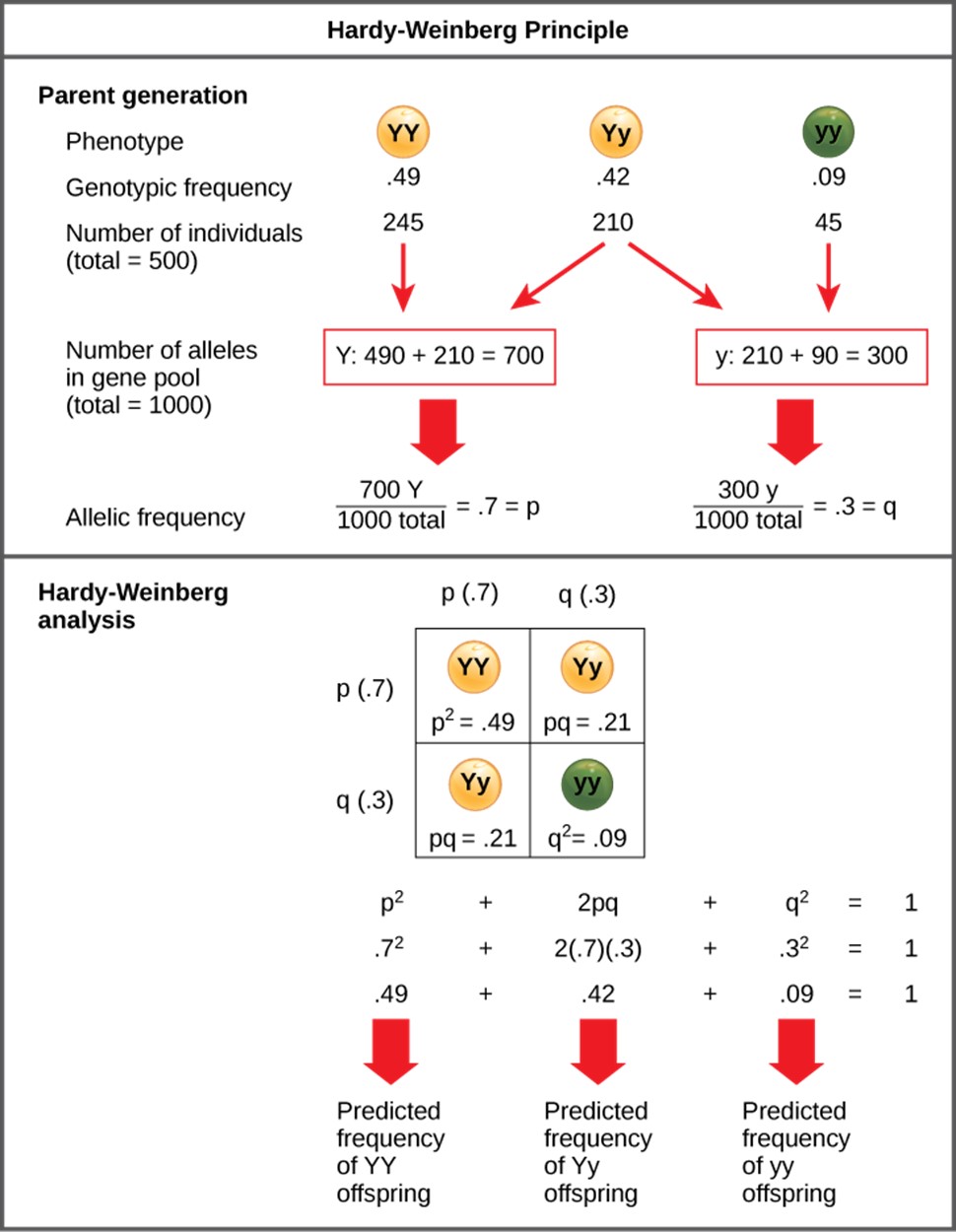
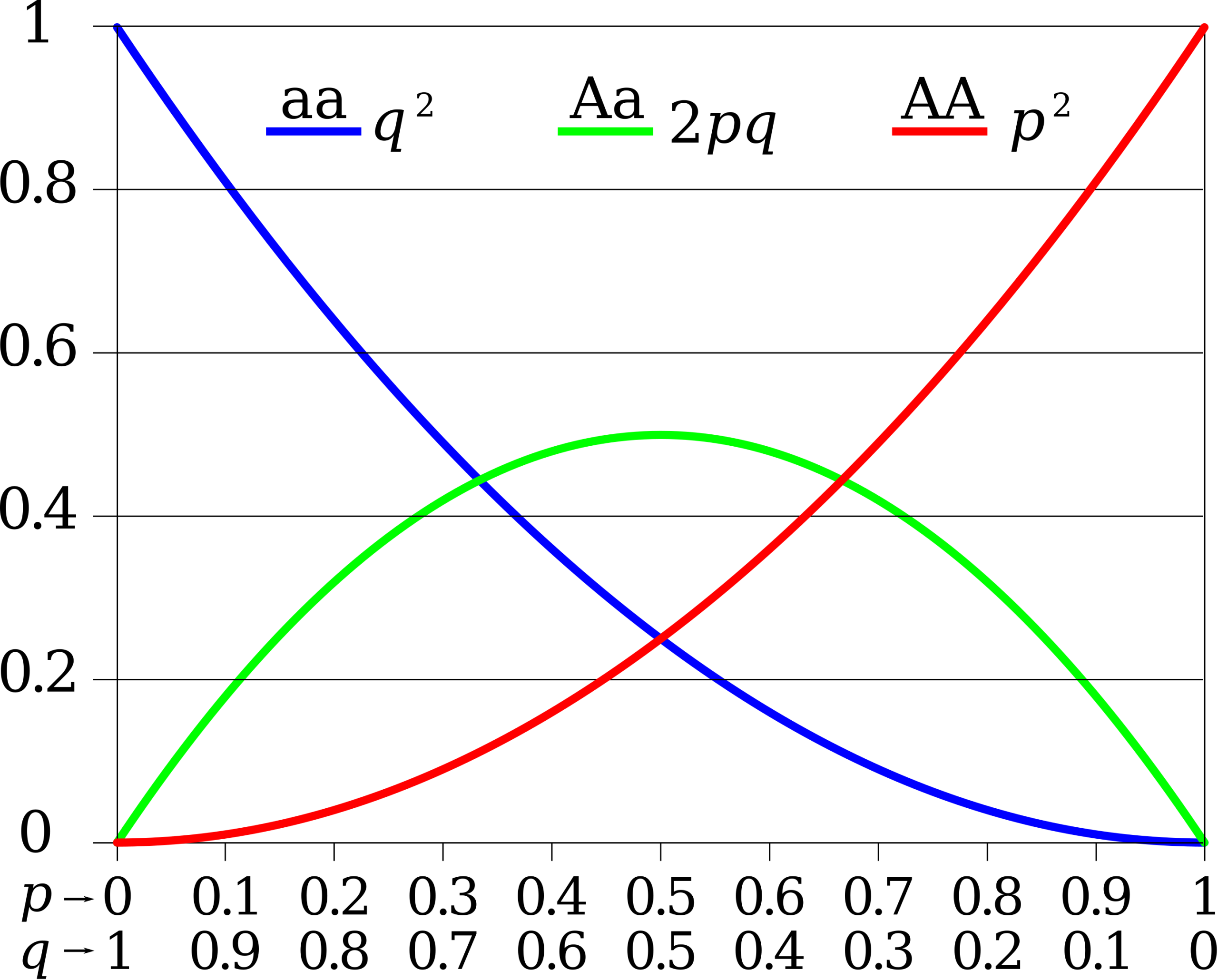
Since each individual carries two alleles per gene, if the allele frequencies (p and q) are known, predicting the frequencies of these genotypes is a simple mathematical calculation to determine the probability of getting these genotypes if two alleles are drawn at random from the gene pool. So in the above scenario, an individual pea plant could be pp (YY), and thus produce yellow peas; pq (Yy), also yellow; or qq (yy), and thus producing green peas (Figure 16.1.1). In other words, the frequency of pp individuals is simply p2; the frequency of pq individuals is 2pq; and the frequency of qq individuals is q2. And, again, if p and q are the only two possible alleles for a given trait in the population, these genotype frequencies will sum to one: p2 + 2pq + q2 = 1 (Figure 16.1.2).
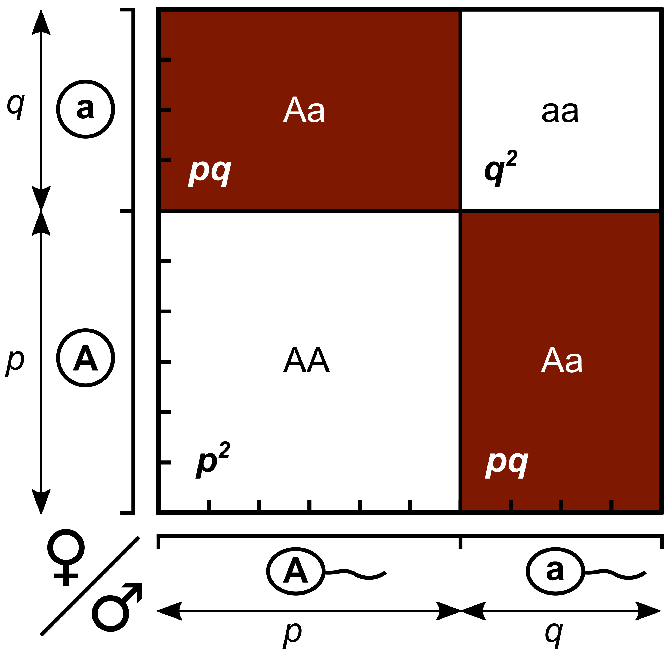
Another way to visualize the relationship between allele frequency and genotype frequency is a Punnett Square for Populations (Figure 16.1.3). We can use these diagrams to help illustrate how predicted allele frequencies translate into predicted genotype frequencies across an entire population under the assumptions of the Hardy-Weinberg equilibrium (large, randomly mating population). For the gene with two alleles shown in Figure 16.1.2 (e.g., A and a), if the frequency of A is p and a is q.
In the “Population Punnett Square” shown in Figure 16.1.3, the length of p and q corresponds to allele frequencies (here p = 0.6, q = 0.4). Then area of rectangle represents predicted genotype frequencies (thus AA:Aa:aa = 0.36:0.48:0.16).
In theory, if a population is at equilibrium—that is, no evolutionary forces are acting upon it—generation after generation would have the same gene pool and genetic structure, and these equations would all hold true all of the time. Thus, when the Hardy-Weinberg equation is used in population genetics, it is assumed that a constant allele frequency will be maintained over time. For this to occur it is implied that:
- The population is large.
- There is random mating.
- There is no mutation.
- There is no gene flow (immigration or emigration).
- There is no natural selection or allele-specific mortality.
Of course, even Hardy and Weinberg recognized that no natural population is immune to evolution. Populations in nature are constantly changing in genetic makeup due to drift, mutation, possibly migration, and selection. As a result, the only way to determine the exact distribution of phenotypes in a population is to go out and count them. The Hardy-Weinberg principle gives scientists a mathematical baseline of a non-evolving population to which they can compare evolving populations and thereby infer what evolutionary forces might be at play. If the frequencies of alleles or genotypes deviate from the value expected from the Hardy-Weinberg equation, then the population is evolving.
This video is a nice overview of Hardy-Weinberg equilibrium.
Video 16.1.1. Hardy-Weinberg Equilibrium by Amoeba Sisters
Violations of Hardy-Weinberg
Remember, that the Hardy-Weinberg principle posits that if a population is not affected by mutation, selection, migration, or genetic drift, and if random mating occurs, the frequencies of alleles and genotypes will remain in equilibrium across generations. In this idealized state, the frequencies of two alleles “A” (dominant) and “a” (recessive) are represented by “p” and “q,” respectively. The principle provides a mathematical formula to predict genotype frequencies:
p2 + 2pq + q2 = 1
where:
- p² represents the proportion of individuals with the homozygous dominant genotype (AA)
- 2pq represents the proportion of individuals with the heterozygous genotype (Aa)
- q² represents the proportion of individuals with the homozygous recessive genotype (aa)
This model assumes that the sum of all allele frequencies equals 1 (i.e., p + q = 1).
In evolutionary biology, the Hardy-Weinberg principle provides a theoretical baseline against which real-world genetic data can be compared. By analyzing deviations (that is, violations) from equilibrium, researchers can infer the presence of evolutionary forces or population-level changes.
Natural Selection
If certain genotypes are found at higher or lower frequencies than expected, this can indicate that natural selection is favoring or disfavoring specific alleles. For instance, in a changing environment, certain traits may confer a selective advantage, leading to changes in allele frequencies.
Genetic Drift
Small, isolated populations are particularly prone to random fluctuations in allele frequencies, known as genetic drift. Comparing genetic data to the Hardy-Weinberg equilibrium helps identify the impact of drift, which can lead to reduced genetic diversity or fixation of alleles.
Gene Flow
Migration between populations can introduce new alleles and homogenize genetic differences. Significant deviations from expected allele frequencies can reveal historical or ongoing migration events that impact local genetic structure.
Non-Random Mating
Mate choice preferences, inbreeding, or assortative mating can alter genotype frequencies, often increasing the proportion of homozygous individuals. These patterns can be detected through a Hardy-Weinberg equilibrium analysis.
Mutation
Although mutations are relatively rare, they provide the raw genetic material for evolution. If new mutations confer an adaptive advantage, they may increase in frequency over time, creating a noticeable deviation from Hardy-Weinberg expectations.
Population Bottlenecks and Founder Effects
Events like population bottlenecks or founder effects can drastically alter genetic variation. Comparing the genetic composition of populations before and after such events reveals the long-term impacts on allele frequencies.
This video has some nice examples of violations of Hardy-Weinberg in the study population of genetics.
Video 16.1.2. Microevolution: What’s An Allele Got to Do with It?: Crash Course Biology #12 by CrashCourse
Use this online calculator [New Tab] to determine the genetic structure of a population (relationship between allele and genotype frequencies).
Hardy-Weinberg Examples
Let’s take a look at how to solve some two-allele problems together. First, If you know the relationship between two alleles, and there is complete dominance of one over the other, then you can start with the recessive allele, because there is only one genotype to express the recessive version of the trait. With the dominant version of a trait there are two possible genotypes—homozygous dominant and heterozygous—which complicates things a bit, so we wait to determine what is going on with these genotypes until after we figure out the recessive.
Second, remember that a genotype or expression of a trait is dictated by two alleles and therefore the equation that deals with 2 alleles is for traits, individuals, genotypes. That is the expression p2 + 2pq + q2 = 1 will deal with genotypes and traits you can see (like black cats, or crooked fingers, etc.). If you are trying to determine an allele, then you just focus on one piece of information (for example, “p” for the most frequent allele).
Example #1
A population of crickets is composed of both loud chirpers and soft chirpers. This trait is determined by genes, with the allele coding for loud chirping being dominant to the one coding for soft chirping.
There are 48 loud chirpers and 14 soft chirpers in the population. What percentage of crickets is heterozygous for loud chirping?
Step 1: Start with the recessive allele and its corresponding phenotype
We need to know what % of the population are soft chirpers. Fourteen crickets out of a total of 62 animals. Since these are individuals and since it is a genotype we are looking at q2. That means 14/62 or 0.225 are soft chirpers.
Step 2: What is the recessive allele frequency?
Since 0.225 is q2, we can take the square root of this to get q. This value is 0.474.
Step 3: Now that we have the q (recessive) allele frequency, determine the p (dominant) allele frequency.
Use the equation p + q = 1 and rearrange to be p = 1 – q
We know that q is 0.474 so plug this in
p = 1 – 0.474 = 0.526
Step 4: Determine what part of the equation you need to solve for and then answer the question
We need to know what the heterozygous frequency is so we are looking at 2pq
We have p and q determined already so we just need to plug in the values.
2 X 0.526 X 0.474 = 0.498
This means that ~50% (rounding up) of the cricket population is heterozygous for loud chirping.
Example #2
In a population of 162 rabbits, 34 of them express a recessive trait. What is the allelic frequency for this trait? Assuming Hardy-Weinberg equilibrium, how many rabbits would you expect to have the recessive trait the following year when 250 rabbits are present?
Step 1: Start with the recessive and find the recessive allele frequency
34 out of 162 have the recessive genotype or trait. That means that 0.209 or ~21% of the rabbits have this recessive trait. This is the q2 value.
To find the allelic frequency, you need to take the square root of 0.21, which is 0.46. This is q.
Step 2: Apply this frequency to determine the prediction for the following year
Remember 0.46 is q (allele) and 0.21 is q2 (genotype). If we have 250 rabbits, we can use the percentage and apply it.
That is, we expect ~21% of the rabbits to have the recessive trait.
So 0.21 X 250 rabbits = 52.5 or 53 rabbits
If there is no evolution and equilibrium remains, we expect that 53 rabbits out of the 250 will be exhibiting the recessive trait
(As a double-check, you can take 53 out of 250 and you will find that 0.21 frequency for the recessive trait. This tells us we did the problem correctly).
In theory, if a population is at equilibrium—that is, there are no evolutionary forces acting upon it—generation after generation would have the same gene pool and genetic structure, and these equations would all hold true all of the time. Of course, even Hardy and Weinberg recognized that no natural population is immune to evolution. Populations in nature are constantly changing in genetic makeup due to drift, mutation, possibly migration, and selection. As a result, the only way to determine the exact distribution of phenotypes in a population is to go out and count them. But the Hardy-Weinberg principle gives scientists a mathematical baseline of a non-evolving population to which they can compare evolving populations and thereby infer what evolutionary forces might be at play. If the frequencies of alleles or genotypes deviate from the value expected from the Hardy-Weinberg equation, then the population is evolving.
Section Summary
The modern synthesis of evolutionary theory grew out of the cohesion of Darwin’s, Wallace’s, and Mendel’s thoughts on evolution and heredity, along with the more modern study of population genetics. It describes the evolution of populations and species, from small-scale changes among individuals to large-scale changes over paleontological time periods. To understand how organisms evolve, scientists can track populations’ allele frequencies over time. If they differ from generation to generation, scientists can conclude that the population is not in Hardy-Weinberg equilibrium, and is thus evolving.
Practice Questions
Free Response Questions
Glossary
- allele frequency
- (also, gene frequency) rate at which a specific allele appears within a population
- founder effect
- event that initiates an allele frequency change in part of the population, which is not typical of the original population
- gene pool
- all of the alleles carried by all of the individuals in the population
- genetic structure
- distribution of the different possible genotypes in a population
- macroevolution
- broader scale evolutionary changes seen over paleontological time
- microevolution
- changes in a population’s genetic structure
- modern synthesis
- overarching evolutionary paradigm that took shape by the 1940s and is generally accepted today
- population genetics
- study of how selective forces change the allele frequencies in a population over time
Figure Descriptions
Figure 16.1.1. The diagram is divided into two sections. The top section, labeled “Parent generation,” shows three genotypes (YY, Yy, and yy) with genotypic frequencies of 0.49, 0.42, and 0.09, corresponding to 245, 210, and 45 individuals out of 500. Red arrows show how the total number of each allele in the population is calculated: 490 Y alleles from YY plus 210 Y alleles from Yy equals 700 total Y alleles; 210 y alleles from Yy plus 90 y alleles from yy equals 300 total y alleles. These are divided by the total alleles in the population (1000) to give p = 0.7 (Y) and q = 0.3 (y). The bottom section, labeled “Hardy-Weinberg analysis,” shows a Punnett square with p (0.7) on the top and left, and q (0.3) on the side. The square contains YY with p² = 0.49, Yy with pq = 0.21 (appearing twice), and yy with q² = 0.09. Below, the equation p² + 2pq + q² = 1 is shown as 0.49 + 0.42 + 0.09 = 1, with red arrows indicating predicted frequencies: YY = 0.49, Yy = 0.42, and yy = 0.09. [Return to Figure 16.1.1]
Figure 16.1.2. The graph has allele frequencies (p and q) on the horizontal axis ranging from 0 to 1, and expected genotype frequencies on the vertical axis ranging from 0 to 1. Three curves are shown: a blue decreasing curve for p² (homozygous dominant genotype), a red increasing curve for q² (homozygous recessive genotype), and a green bell-shaped curve for 2pq (heterozygous genotype) that peaks at p = q = 0.5. The intersection points of the curves show where genotype frequencies change relative dominance as allele frequencies shift. [Return to Figure 16.1.2]
Figure 16.1.3. Diagram of a Punnett square labeled “Population Punnett Square.” The left side represents female gametes and the top represents male gametes. The vertical axis shows allele A at frequency p and allele a at frequency q, while the horizontal axis shows the same alleles and frequencies for males. The square’s four boxes represent genotype frequencies: top left is Aa (pq, shaded dark red), top right is aa (q², white), bottom left is AA (p², white), and bottom right is Aa (pq, shaded dark red). The lengths of p and q correspond to allele frequencies, and the areas of the boxes correspond to genotype frequencies. [Return to Figure 16.1.3]
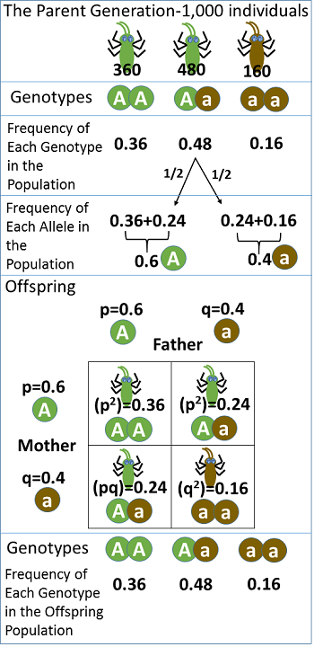
Figure 16.1.4. The diagram is divided into three sections. In the top section (parent generation: 1,000 individuals), three genotype groups are depicted using small green-and-black insect-like creatures to represent AA (solid green body, 360 individuals, frequency 0.36), Aa (half green, half brown body, 480 individuals, frequency 0.48), and aa (solid brown body, 160 individuals, frequency 0.16). The calculation of allele frequencies is shown as A = 0.36 + 0.24 = 0.6 and a = 0.24 + 0.16 = 0.4. In the middle section (Offspring), a Punnett square displays the mating between a father (p = 0.6 A, q = 0.4 a) and a mother (p = 0.6 A, q = 0.4 a), with the same insect-like creatures illustrating the resulting genotypes: AA (p² = 0.36, solid green), Aa (pq = 0.24 in two boxes, half green and half brown), and aa (q² = 0.16, solid brown). The bottom section (Offspring Genotypes) shows these same insects in proportions identical to the parent generation—AA = 0.36, Aa = 0.48, and aa = 0.16—illustrating Hardy-Weinberg equilibrium. [Return to Figure 16.1.4]
Figure 16.1.5. The diagram is divided into two sections. The top section, labeled “Parent generation,” shows three genotypes (YY, Yy, and yy) with genotypic frequencies of 0.49, 0.42, and 0.09, corresponding to 245, 210, and 45 individuals out of 500. Red arrows show how the total number of each allele in the population is calculated: 490 Y alleles from YY plus 210 Y alleles from Yy equals 700 total Y alleles; 210 y alleles from Yy plus 90 y alleles from yy equals 300 total y alleles. These are divided by the total alleles in the population (1000) to give p = 0.7 (Y) and q = 0.3 (y). The bottom section, labeled “Hardy-Weinberg analysis,” shows a Punnett square with p (0.7) on the top and left, and q (0.3) on the side. The square contains YY with p² = 0.49, Yy with pq = 0.21 (appearing twice), and yy with q² = 0.09. Below, the equation p² + 2pq + q² = 1 is shown as 0.49 + 0.42 + 0.09 = 1, with red arrows indicating predicted frequencies: YY = 0.49, Yy = 0.42, and yy = 0.09. [Return to Figure 16.1.5]
References
Hanania, S., Hassawi, D., & Irshaid, N. (2007). Allele frequency and molecular genotypes of ABO blood group system in a Jordanian population. Journal of Medical Sciences, 7:51–58, doi:10.3923/jms.2007.51.58.
Licenses and Attributions
This chapter, “Population Genetics,” by Elizabeth Dahlhoff, is adapted from chapters in the “Evolution” section in Introductory Biology: Ecology, Evolution, and Biodiversity by Erica Kosal (North Carolina State University) under a CC BY-NC 4.0 license. This work is licensed under a CC BY-NC 4.0 license.
Media Attributions
- ns4
- Hardy-Weinberg
- Hardy–Weinberg_law_-_Punnett_square.svg
- Hartsock_Hardy_Weinberg_Example © Angela Hartsock is licensed under a CC0 (Creative Commons Zero) license
