Chapter 8 Advanced Theories of Covalent Bonding
8.4 Molecular Orbital Theory
Learning Objectives
By the end of this section, you will be able to:
- Outline the basic quantum-mechanical approach to deriving molecular orbitals from atomic orbitals
- Describe traits of bonding and antibonding molecular orbitals
- Calculate bond orders based on molecular electron configurations
- Write molecular electron configurations for first- and second-row diatomic molecules
- Relate these electron configurations to the molecules’ stabilities and magnetic properties
For almost every covalent molecule that exists, we can now draw the Lewis structure, predict the electron-pair geometry, predict the molecular geometry, and come close to predicting bond angles. However, one of the most important molecules we know, the oxygen molecule O2, presents a problem with respect to its Lewis structure. We would write the following Lewis structure for O2:

This electronic structure adheres to all the rules governing Lewis theory. There is an O=O double bond, and each oxygen atom has eight electrons around it. However, this picture is at odds with the magnetic behavior of oxygen. By itself, O2 is not magnetic, but it is attracted to magnetic fields. Thus, when we pour liquid oxygen past a strong magnet, it collects between the poles of the magnet and defies gravity, as in Figure 8.1. Such attraction to a magnetic field is called paramagnetism, and it arises in molecules that have unpaired electrons. And yet, the Lewis structure of O2 indicates that all electrons are paired. How do we account for this discrepancy?
Magnetic susceptibility measures the force experienced by a substance in a magnetic field. When we compare the weight of a sample to the weight measured in a magnetic field (Figure 8.28), paramagnetic samples that are attracted to the magnet will appear heavier because of the force exerted by the magnetic field. We can calculate the number of unpaired electrons based on the increase in weight.
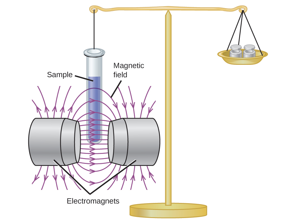
Experiments show that each O2 molecule has two unpaired electrons. The Lewis-structure model does not predict the presence of these two unpaired electrons. Unlike oxygen, the apparent weight of most molecules decreases slightly in the presence of an inhomogeneous magnetic field. Materials in which all of the electrons are paired are diamagnetic and weakly repel a magnetic field. Paramagnetic and diamagnetic materials do not act as permanent magnets. Only in the presence of an applied magnetic field do they demonstrate attraction or repulsion.
Link to Learning
Water, like most molecules, contains all paired electrons. Objects that contain a large percentage of water therefore demonstrate diamagnetic behavior. For example, if you place a strawberry in a powerful magnetic field, it will levitate!
The same effect can be demonstrated on living creatures, provided their mass is small enough!
Molecular orbital theory (MO theory) provides an explanation of chemical bonding that accounts for the paramagnetism of the oxygen molecule. It also explains the bonding in a number of other molecules, such as violations of the octet rule and more molecules with more complicated bonding (beyond the scope of this text) that are difficult to describe with Lewis structures. Additionally, it provides a model for describing the energies of electrons in a molecule and the probable location of these electrons. Unlike valence bond theory, which uses hybrid orbitals that are assigned to one specific atom, MO theory uses the combination of atomic orbitals to yield molecular orbitals that are delocalized over the entire molecule rather than being localized on its constituent atoms. MO theory also helps us understand why some substances are electrical conductors, others are semiconductors, and still others are insulators. Table 8.2 summarizes the main points of the two complementary bonding theories. Both theories provide different, useful ways of describing molecular structure.
|
Valence Bond Theory |
Molecular Orbital Theory |
|---|---|
|
considers bonds as localized between one pair of atoms |
considers electrons delocalized throughout the entire molecule |
|
creates bonds from the overlap of atomic orbitals (s, p, d, and so on) and hybrid orbitals (sp, sp2, sp3, and so on) |
combines atomic orbitals to form molecular orbitals (σ, σ*, π, π*) |
|
forms σ or π bonds |
creates bonding and antibonding interactions based on which orbitals are filled |
|
predicts molecular shape based on the number of regions of electron density |
predicts the arrangement of electrons in molecules |
|
needs multiple structures to describe resonance |
|
Molecular orbital theory describes the distribution of electrons in molecules in much the same way that the distribution of electrons in atoms is described using atomic orbitals. Using quantum mechanics, the behavior of an electron in a molecule is still described by a wave function, Ψ, analogous to the behavior in an atom. Just like electrons around isolated atoms, electrons around atoms in molecules are limited to discrete (quantized) energies. The region of space in which a valence electron in a molecule is likely to be found is called a molecular orbital (Ψ2). Like an atomic orbital, a molecular orbital is full when it contains two electrons with opposite spin.
We will consider the molecular orbitals in molecules composed of two identical atoms (H2 or Cl2, for example). Such molecules are called homonuclear diatomic molecules. In these diatomic molecules, several types of molecular orbitals occur.
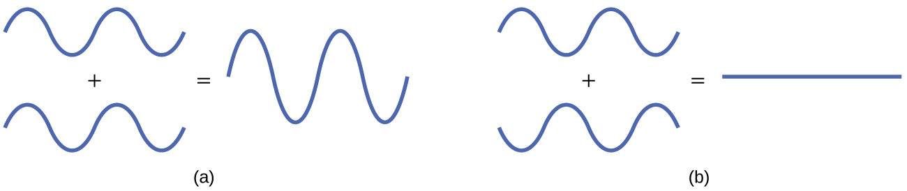
The mathematical process of combining atomic orbitals to generate molecular orbitals is called the linear combination of atomic orbitals (LCAO). The wave function describes the wavelike properties of an electron. Molecular orbitals are combinations of atomic orbital wave functions. Combining waves can lead to constructive interference, in which peaks line up with peaks, or destructive interference, in which peaks line up with troughs (Figure 8.29). In orbitals, the waves are three dimensional, and they combine with in-phase waves producing regions with a higher probability of electron density and out-of-phase waves producing nodes, or regions of no electron density.
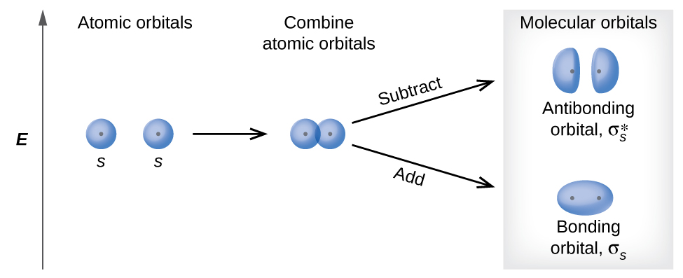
There are two types of molecular orbitals that can form from the overlap of two atomic s orbitals on adjacent atoms. The two types are illustrated in Figure 8.30. The in-phase combination produces a lower energy σs molecular orbital (read as "sigma-s") in which most of the electron density is directly between the nuclei. The out-of-phase addition (which can also be thought of as subtracting the wave functions) produces a higher energy σs* molecular orbital (read as "sigma-s-star") molecular orbital in which there is a node between the nuclei. The asterisk signifies that the orbital is an antibonding orbital. Electrons in a σs orbital are attracted by both nuclei at the same time and are more stable (of lower energy) than they would be in the isolated atoms. Adding electrons to these orbitals creates a force that holds the two nuclei together, so we call these orbitals bonding orbitals. Electrons in the σs* orbitals are located well away from the region between the two nuclei. The attractive force between the nuclei and these electrons pulls the two nuclei apart. Hence, these orbitals are called antibonding orbitals. Electrons fill the lower-energy bonding orbital before the higher-energy antibonding orbital, just as they fill lower-energy atomic orbitals before they fill higher-energy atomic orbitals.
Link to Learning
Watch the video below to help visualize how atomic orbitals combine to form various molecular orbitals.
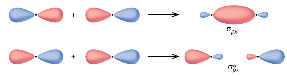
In p orbitals, the wave function gives rise to two lobes with opposite phases, analogous to how a two-dimensional wave has both parts above and below the average. We indicate the phases by shading the orbital lobes different colors. When orbital lobes of the same phase overlap, constructive wave interference increases the electron density. When regions of opposite phase overlap, the destructive wave interference decreases electron density and creates nodes. When p orbitals overlap end to end, they create σ and σ* orbitals (Figure 8.31). If two atoms are located along the x-axis in a Cartesian coordinate system, the two px orbitals overlap end to end and form σpx (bonding) and σpx* (antibonding) (read as "sigma-p-x" and "sigma-p-x star," respectively). Just as with s-orbital overlap, the asterisk indicates the orbital with a node between the nuclei, which is a higher-energy, antibonding orbital.
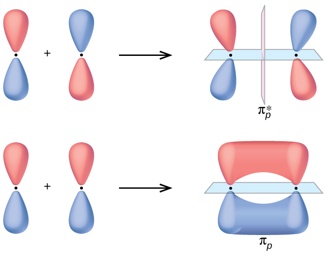
The side-by-side overlap of two p orbitals gives rise to a pi (π) bonding molecular orbital and a π* antibonding molecular orbital, as shown in Figure 8.32. In valence bond theory, we describe π bonds as containing a nodal plane containing the internuclear axis and perpendicular to the lobes of the p orbitals, with electron density on either side of the node. In molecular orbital theory, we describe the π orbital by this same shape, and a π bond exists when this orbital contains electrons. Electrons in this orbital interact with both nuclei and help hold the two atoms together, making it a bonding orbital. For the out-of-phase combination, there are two nodal planes created, one along the internuclear axis and a perpendicular one between the nuclei.
In the molecular orbitals of diatomic molecules, each atom also has two sets of p orbitals oriented side by side (py and pz), so these four atomic orbitals combine pairwise to create two π orbitals and two π* orbitals. The πpy and πpy* orbitals are oriented at right angles to the πpz and πpz* orbitals. Except for their orientation, the πpy and πpz orbitals are identical and have the same energy; they are degenerate orbitals. The πpy* and πpz* antibonding orbitals are also degenerate and identical except for their orientation. A total of six molecular orbitals results from the combination of the six atomic p orbitals in two atoms: σpx and σpx*, πpy and πpy*, πpz and πpz*.
Example 8.5. Molecular Orbitals
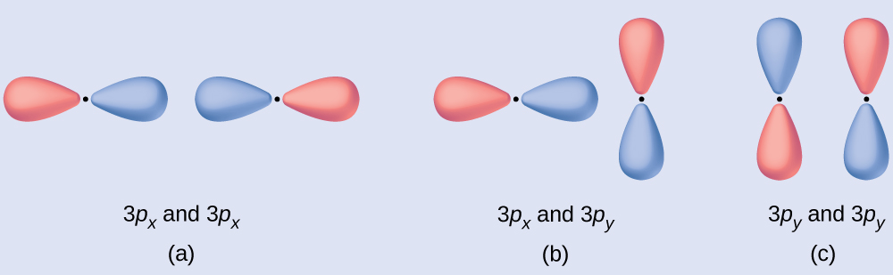
Predict what type (if any) of molecular orbital would result from adding the wave functions so each pair of orbitals shown overlap. The orbitals are all similar in energy.
Click here for the answers!
(a) Is an in-phase combination, resulting in a σ3p orbital.
(b) Will not result in a new orbital because the in-phase component (bottom) and out-of-phase component (top) cancel out. Only orbitals with the correct alignment can combine.
(c) Is an out-of-phase combination, resulting in a π3p* orbital.
Check Your Learning

Click here to see this MO with the node labeled!

Portrait of a Chemist
Walter Kohn, Nobel Laureate
Walter Kohn (Figure 8.33) is an Austrian-American theoretical physicist who studied the electronic structure of solids. His work combined the principles of quantum mechanics with advanced mathematical techniques. This technique, called density functional theory, makes it possible to compute properties of molecular orbitals, including their shape and energies. Kohn and mathematician John Pople were awarded the Nobel Prize in Chemistry in 1998 for their contributions to our understanding of electronic structure. Kohn also made significant contributions to the physics of semiconductors.
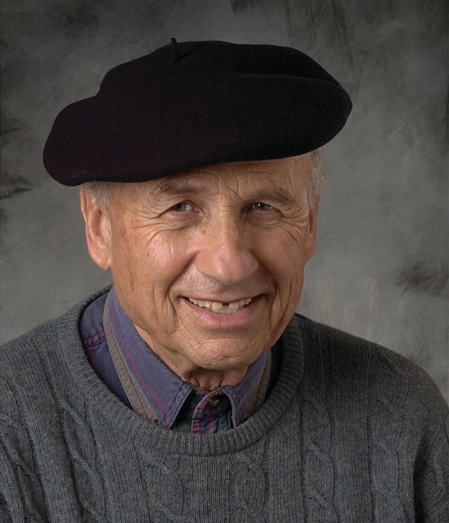
Kohn’s biography has been remarkable outside the realm of physical chemistry as well. He was born in Austria, and during World War II he was part of the Kindertransport program that rescued 10,000 children from the Nazi regime. His summer jobs included discovering gold deposits in Canada and helping Polaroid explain how its instant film worked. Dr. Kohn passed away in 2016 at the age of 93.
How Sciences Interconnect
Computational Chemistry in Drug Design
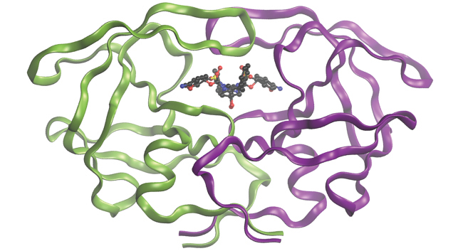
While the descriptions of bonding described in this chapter involve many theoretical concepts, they also have many practical, real-world applications. For example, drug design is an important field that uses our understanding of chemical bonding to develop pharmaceuticals. This interdisciplinary area of study uses biology (understanding diseases and how they operate) to identify specific targets, such as a binding site that is involved in a disease pathway. By modeling the structures of the binding site and potential drugs, computational chemists can predict which structures can fit together and how effectively they will bind (Figure 8.34). Thousands of potential candidates can be narrowed down to a few of the most promising candidates. These candidate molecules are then carefully tested to determine side effects, how effectively they can be transported through the body, and other factors. Dozens of important new pharmaceuticals have been discovered with the aid of computational chemistry, and new research projects are underway.
Molecular Orbital Energy Diagrams
The relative energy levels of atomic and molecular orbitals are typically shown in a molecular orbital diagram (Figure 8.35). For a diatomic molecule, the atomic orbitals of one atom are shown on the left, and those of the other atom are shown on the right. Each horizontal line represents one orbital that can hold two electrons. The molecular orbitals formed by the combination of the atomic orbitals are shown in the center. Dashed lines show which of the atomic orbitals combine to form the molecular orbitals. For each pair of atomic orbitals that combine, one lower-energy (bonding) molecular orbital and one higher-energy (antibonding) orbital result.
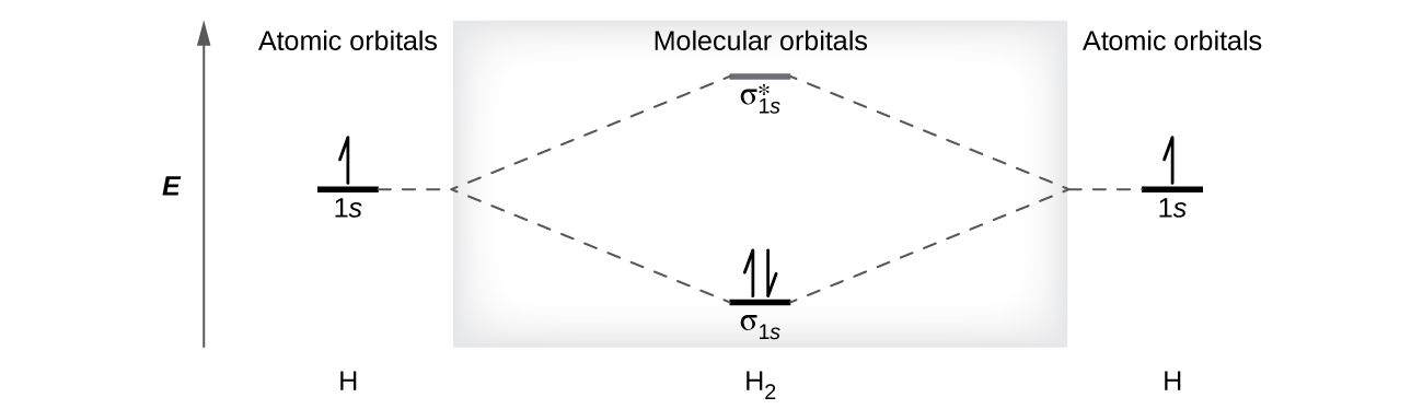
We predict the distribution of electrons in these molecular orbitals by filling the orbitals in the same way that we fill atomic orbitals, by the Aufbau principle. Lower-energy orbitals fill first, electrons spread out among degenerate orbitals before pairing, and each orbital can hold a maximum of two electrons with opposite spins. Just as we write electron configurations for atoms, we can write the molecular electronic configuration by listing the orbitals with superscripts indicating the number of electrons present. Both electrons in the H2 molecule are in the σ1s bonding orbital (Figure 8.35); the electron configuration is therefore σ1s2.
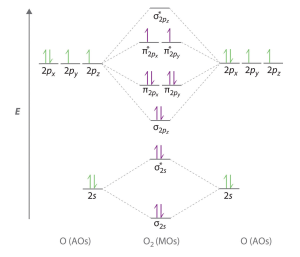
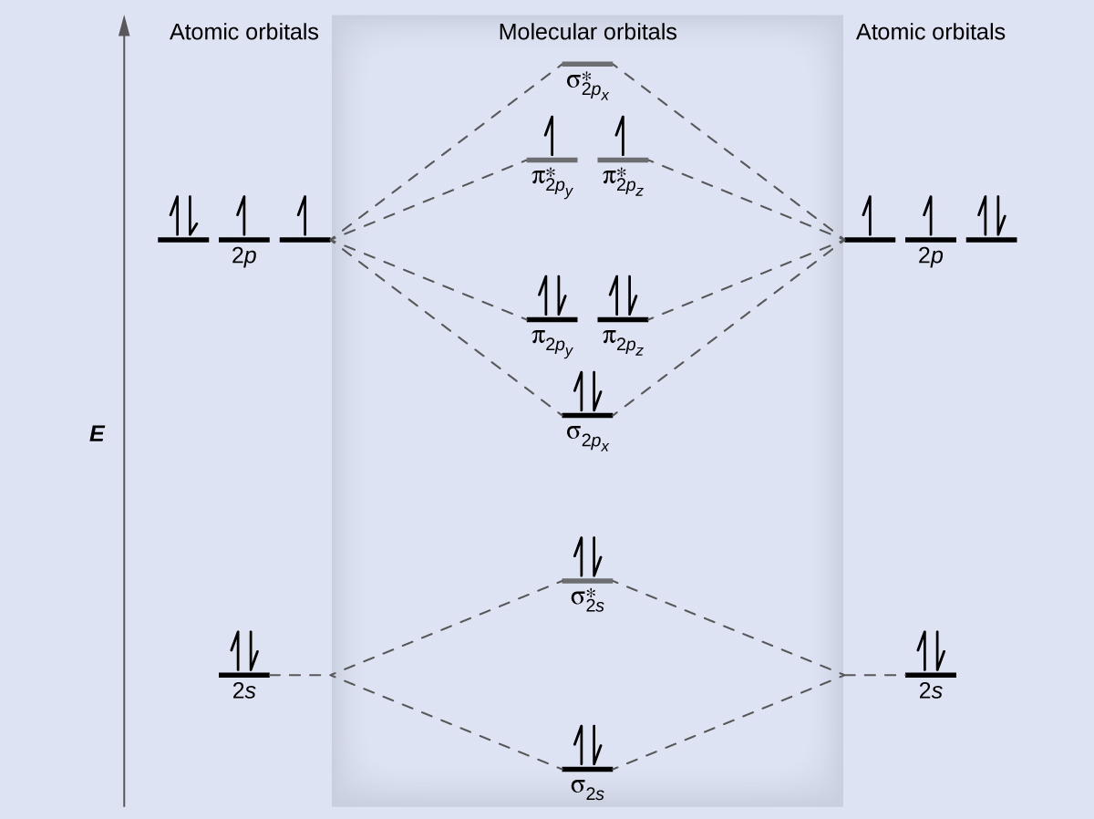
Figure 8.36 shows a molecular orbital diagram for O2. We observe that combining the six 2p atomic orbitals results in three bonding orbitals (one σ and two π) and three antibonding orbitals (one σ* and two π*). The electron configuration of O2 is (σ2s)2(σ2s*)2(σ2px)2(π2py, π2pz)4(π2py*, π2pz*)2. For clarity, we place parentheses around molecular orbitals with the same energy. Note that it is common to omit the core electrons from molecular orbital diagrams and configurations and include only the valence electrons.
Bond Order
The filled molecular orbital diagram shows the number of electrons in both bonding and antibonding molecular orbitals. The net contribution of the electrons to the bond strength of a molecule is identified by determining the bond order that results from the filling of the molecular orbitals by electrons.
When using Lewis structures to describe the distribution of electrons in molecules, we define bond order as the number of bonding pairs of electrons between two atoms. Thus a single bond has a bond order of 1, a double bond has a bond order of 2, and a triple bond has a bond order of 3. We define bond order differently when we use the molecular orbital description of the distribution of electrons, but the resulting bond order is usually the same. The MO technique is more accurate and can handle cases when the Lewis structure method fails, but both methods describe the same phenomenon.
In the molecular orbital model, an electron contributes to a bonding interaction if it occupies a bonding orbital and it contributes to an antibonding interaction if it occupies an antibonding orbital. The bond order is calculated by subtracting the destabilizing (antibonding) electrons from the stabilizing (bonding) electrons. Since a bond consists of two electrons, we divide by two to get the bond order. We can determine bond order with the following equation:
[latex]bond \; order = \frac {(number \; of \; bonding \; electrons) - (number \; of \; antibonding \; electrons)}{2}[/latex]
The order of a covalent bond is a guide to its strength; a bond between two given atoms becomes stronger as the bond order increases (Table 8.1). If the distribution of electrons in the molecular orbitals between two atoms is such that the resulting bond would have a bond order of zero, a stable bond does not form. We next look at some specific examples of MO diagrams and bond orders.
Bonding in Diatomic Molecules
A dihydrogen molecule (H2) forms from two hydrogen atoms (Figure 8.35). When the atomic orbitals of the two atoms combine, the electrons occupy the molecular orbital of lowest energy, the σ1s bonding orbital. The σ1s orbital that contains both electrons is lower in energy than either of the two 1s atomic orbitals. A dihydrogen molecule, H2, therefore readily forms because the energy of a H2 molecule is lower than that of two H atoms.
A dihydrogen molecule contains two bonding electrons and no antibonding electrons so we have:
Because the bond order for the H–H bond is equal to 1, the bond is a single bond.
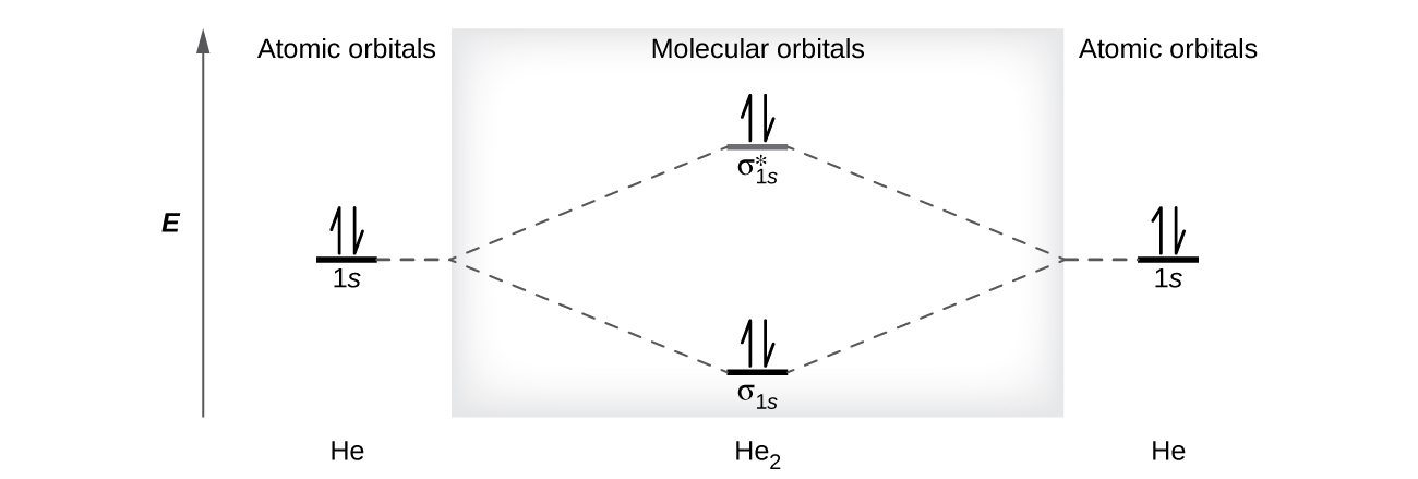
A helium atom has two electrons, both of which are in its 1s orbital. Two helium atoms do not combine to form a dihelium molecule, He2, with four electrons, because the stabilizing effect of the two electrons in the lower-energy bonding orbital would be offset by the destabilizing effect of the two electrons in the higher-energy antibonding molecular orbital. We would write the hypothetical electron configuration of He2 as (σ1s)2(σ1s*)2as in Figure 8.37. The net energy change would be zero, so there is no driving force for helium atoms to form the diatomic molecule. In fact, helium exists as discrete atoms rather than as diatomic molecules. The bond order in a hypothetical dihelium molecule would be zero.
A bond order of zero indicates that no bond is formed between two atoms.
The Diatomic Molecules of the Second Period
Eight possible homonuclear diatomic molecules might be formed by the atoms of the second period of the periodic table: Li2, Be2, B2, C2, N2, O2, F2, and Ne2. Below, we investigate their molecular orbital diagrams.
As we saw in valence bond theory, σ bonds are generally more stable than π bonds formed from degenerate atomic orbitals. Similarly, in molecular orbital theory, σ orbitals are usually more stable than π orbitals. However, this is not always the case. The MOs for the valence orbitals of the second period are shown in Figure 8.38. Looking at Ne2 molecular orbitals, we see that the order is consistent with the generic diagram shown in the previous section. However, for atoms with three or fewer electrons in the p orbitals (Li through N) we observe a different pattern, in which the σp orbital is higher in energy than the πp set. Obtain the molecular orbital diagram for a homonuclear diatomic ion by adding or subtracting electrons from the diagram for the neutral molecule.
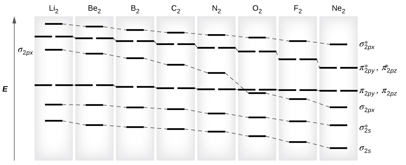
This switch in orbital ordering occurs because of a phenomenon called s-p mixing. s-p mixing does not create new orbitals; it merely influences the energies of the existing molecular orbitals. The σs wavefunction mathematically combines with the σp wavefunction, with the result that the σs orbital becomes more stable, and the σp orbital becomes less stable (Figure 8.39). Similarly, the antibonding orbitals also undergo s-p mixing, with the σs* becoming more stable and the σp* becoming less stable.
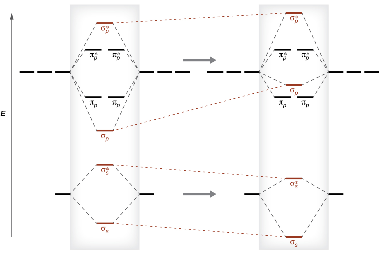
This s-p mixing occurs when the s and p orbitals have similar energies. The energy difference between 2s and 2p orbitals in O, F, and Ne is greater than that in Li, Be, B, C, and N. Because of this, O2, F2, and Ne2 exhibit negligible s-p mixing (not sufficient to change the energy ordering), and their MO diagrams follow the normal pattern, as shown in Figure 8.38. All of the other period 2 diatomic molecules do have s-p mixing, which leads to the pattern where the σp orbital is raised above the πp set.
Using the MO diagrams shown in Figure 8.38, we can add in the electrons and determine the molecular electron configuration and bond order for each of the diatomic molecules (Table 8.3). We predict valence molecular orbital electron configurations just as we predict electron configurations of atoms. Valence electrons are assigned to valence molecular orbitals with the lowest possible energies. Consistent with Hund’s rule, whenever there are two or more degenerate molecular orbitals, electrons fill each orbital of that type singly before any pairing of electrons takes place. As shown in Table 8.3, Be2 and Ne2 molecules would have a bond order of 0, so these molecules do not exist.
|
Molecule |
Electron Configuration |
Bond Order |
|---|---|---|
|
Li2 |
(σ2s)2
|
1 |
|
Be2 (unstable) |
(σ2s)2(σ2s*)2
|
0 |
|
B2 |
(σ2s)2(σ2s*)2(π2py, π2pz)2
|
1 |
|
C2 |
(σ2s)2(σ2s*)2(π2py, π2pz)4
|
2 |
|
N2 |
(σ2s)2(σ2s*)2(π2py, π2pz)4(σ2px)2
|
3 |
|
O2 |
(σ2s)2(σ2s*)2(σ2px)2(π2py, π2pz)4(π2py*, π2pz*)2
|
2 |
|
F2 |
(σ2s)2(σ2s*)2(σ2px)2(π2py, π2pz)4(π2py*, π2pz*)4
|
1 |
|
Ne2 (unstable) |
(σ2s)2(σ2s*)2(σ2px)2(π2py, π2pz)4(π2py*,π2pz*)4(σ2px*)2
|
0 |
The combination of two lithium atoms to form a lithium molecule, Li2, is analogous to the formation of H2, but the atomic orbitals involved are the valence 2s orbitals. Each of the two lithium atoms has one valence electron. Hence, we have two valence electrons available for the σ2s bonding molecular orbital. Because both valence electrons would be in a bonding orbital, we would predict the Li2 molecule to be stable. The molecule is, in fact, present in appreciable concentration in lithium vapor at temperatures near the boiling point of the element. All of the other molecules in Table 8.3 with a bond order greater than zero also form.
The O2 molecule has enough electrons to half fill the π2py*, π2pz* level. We expect the two electrons that occupy these two degenerate orbitals to be unpaired, and this molecular electronic configuration for O2 is in accord with the fact that the oxygen molecule has two unpaired electrons (Figure 8.40). The presence of two unpaired electrons has proved to be difficult to explain using Lewis structures, but molecular orbital theory explains it quite well. In fact, the unpaired electrons of the oxygen molecule provide a strong piece of support for molecular orbital theory.
How Sciences Interconnect
Band Theory
When two identical atomic orbitals on different atoms combine, two molecular orbitals result (Figure 8.30). The bonding orbital is lower in energy than the original atomic orbitals because the atomic orbitals are in-phase in the molecular orbital. The antibonding orbital is higher in energy than the original atomic orbitals because the atomic orbitals are out-of-phase.
In a solid, similar things happen, but on a much larger scale. Remember that even in a small sample there are a huge number of atoms (typically > 1023 atoms), and therefore a huge number of atomic orbitals that may be combined into molecular orbitals. When N valence atomic orbitals, all of the same energy and each containing one (1) electron, are combined, N/2 (filled) bonding orbitals and N/2 (empty) antibonding orbitals will result. Each bonding orbital will show an energy lowering as the atomic orbitals are mostly in-phase, but each of the bonding orbitals will be a little different and have slightly different energies. The antibonding orbitals will show an increase in energy as the atomic orbitals are mostly out-of-phase, but each of the antibonding orbitals will also be a little different and have slightly different energies. The allowed energy levels for all the bonding orbitals are so close together that they form a band, called the valence band. Likewise, all the antibonding orbitals are very close together and form a band, called the conduction band. Figure 8.40 shows the bands for three important classes of materials: insulators, semiconductors, and conductors.
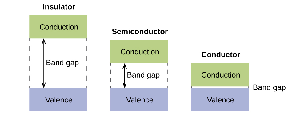
In order to conduct electricity, electrons must move from the filled valence band to the empty conduction band where they can move throughout the solid. The size of the band gap, or the energy difference between the top of the valence band and the bottom of the conduction band, determines how easy it is to move electrons between the bands. Only a small amount of energy is required in a conductor because the band gap is very small. This small energy difference is “easy” to overcome, so they are good conductors of electricity. In an insulator, the band gap is so “large” that very few electrons move into the conduction band; as a result, insulators are poor conductors of electricity. Semiconductors conduct electricity when “moderate” amounts of energy are provided to move electrons out of the valence band and into the conduction band. Semiconductors, such as silicon, are found in many electronics.
Semiconductors are used in devices such as computers, smartphones, and solar cells. Solar cells produce electricity when light provides the energy to move electrons out of the valence band. The electricity that is generated may then be used to power a light or tool, or it can be stored for later use by charging a battery. As of December 2014, up to 46% of the energy in sunlight could be converted into electricity using solar cells.
Example 8.6. Molecular Orbital Diagrams, Bond Order, and Number of Unpaired Electrons
Draw the molecular orbital diagram for the oxygen molecule, O2. From this diagram, calculate the bond order for O2. How does this diagram account for the paramagnetism of O2?
Solution
We draw a molecular orbital energy diagram similar to that shown in Figure 8.38. Each oxygen atom contributes six electrons, so the diagram appears as shown in Figure 8.41.
We calculate the bond order as:
Oxygen's paramagnetism is explained by the presence of two unpaired electrons in the (π2py, π2pz)* molecular orbitals.
Check Your Learning
The main component of air is N2. From the molecular orbital diagram of N2, predict its bond order and whether it is diamagnetic or paramagnetic. (Hint: Consult Figure 8.38 for the unfilled MO diagram.)
Click here for the answers!
N2 has a bond order of 3 and is diamagnetic.
Example 8.7. Ion Predictions with MO Diagrams
Give the molecular orbital configuration for the valence electrons in C22−. Will this ion be stable?
Solution
Looking at the appropriate MO diagram, we see that the π orbitals are lower in energy than the σp orbital. The valence electron configuration for C2 is (σ2s)2(σ2s*)2(π2py, π2pz)4. Adding two more electrons to generate the C22− anion will give a valence electron configuration of (σ2s)2(σ2s*)2(π2py, π2pz)4(σ2px)2. Since this has six more bonding electrons than antibonding, the bond order will be 3, and the ion should be stable.
Check Your Learning
Using Figure 8.38, create a filled MO diagram for the valence electrons of the Be22− ion.
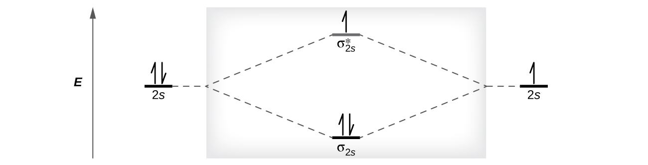
How many unpaired electrons does a Be22− ion have?
two
Is the Be22− ion paramagnetic or diamagnetic?
paramagnetic
Link to Learning
Creating molecular orbital diagrams for molecules with more than two atoms relies on the same basic ideas as the diatomic examples presented here. However, with more atoms, computers are required to calculate how the atomic orbitals combine. See three-dimensional drawings of the molecular orbitals for C6H6.
