6.1 Electromagnetic Energy

The nature of light has been a subject of inquiry since antiquity. In the seventeenth century, Isaac Newton performed experiments with lenses and prisms and was able to demonstrate that white light consists of the individual colors of the rainbow combined together (Figure 6.2). Newton explained his optics findings in terms of a “corpuscular” view of light, in which light was composed of streams of extremely tiny particles traveling at high speeds according to Newton’s laws of motion. Others in the seventeenth century, such as Christiaan Huygens, had shown that optical phenomena such as reflection and refraction could be equally well explained in terms of light as waves travelling at high speed through a medium called “luminiferous aether” that was thought to permeate all space. Early in the nineteenth century, Thomas Young demonstrated that light passing through narrow, closely spaced slits produced interference patterns that could not be explained in terms of Newtonian particles but could be easily explained in terms of waves.

.

Later in the nineteenth century, after James Clerk Maxwell developed his theory of electromagnetic radiation and showed that light was the visible part of a vast spectrum of electromagnetic waves, the particle view of light became thoroughly discredited. By the end of the nineteenth century, scientists viewed the physical universe as roughly comprising two separate domains: matter composed of particles moving according to Newton’s laws of motion, and electromagnetic radiation consisting of waves governed by Maxwell’s equations. Today, these domains are referred to as classical mechanics and classical electrodynamics (or classical electromagnetism). Although there were a few physical phenomena that could not be explained within this framework, scientists at that time were so confident of the overall soundness of this framework that they viewed these aberrations as puzzling paradoxes that would ultimately be resolved somehow within this framework. As we shall see, these paradoxes led to a contemporary framework that intimately connects particles and waves at a fundamental level called wave-particle duality, which has superseded the classical view.

Visible light and other forms of electromagnetic radiation play important roles in chemistry, since they can be used to infer the energies of electrons within atoms and molecules. Much of modern technology is based on electromagnetic radiation. For example, radio waves from a mobile phone, X-rays used by dentists, the energy used to cook food in your microwave, the radiant heat from red-hot objects, and the light from your television screen are forms of electromagnetic radiation that all exhibit wavelike behavior.

Waves

A wave is an oscillation or periodic movement that can transport energy from one point in space to another. Common examples of waves are all around us. Shaking the end of a rope transfers energy from your hand to the other end of the rope, dropping a pebble into a pond causes waves to ripple outward along the water’s surface (Figure 6.3), and the expansion of air that accompanies a lightning strike generates sound waves (thunder) that can travel outward for several miles. In each of these cases, kinetic energy is transferred through matter (the rope, water, or air) while the matter remains essentially in place. An insightful example of a wave occurs in sports stadiums when fans in a narrow region of seats rise simultaneously and stand with their arms raised up for a few seconds before sitting down again while the fans in neighboring sections likewise stand up and sit down in sequence. While this wave can quickly encircle a large stadium in a few seconds, none of the fans actually travel with the wave-they all stay in or above their seats.

.

Waves need not be restricted to travel through matter. As Maxwell showed, electromagnetic waves consist of an electric field oscillating in step with a perpendicular magnetic field, both of which are perpendicular to the direction of travel. These waves can travel through a vacuum at a constant speed of 2.998 × 10⁸ m/s, the speed of light (denoted by c).

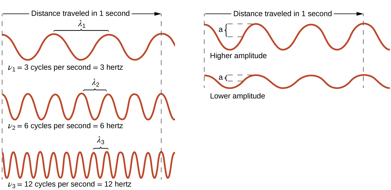
All waves, including forms of electromagnetic radiation, are characterized by a wavelength (denoted by λ, the lowercase Greek letter lambda), a frequency (denoted by ν, the lowercase Greek letter nu), and an amplitude. As can be seen in Figure 6.4, the wavelength is the distance between two consecutive peaks or troughs in a wave (measured in meters in the SI system). Electromagnetic waves have wavelengths that fall within an enormous range-wavelengths of kilometers (10³ m) to picometers (10⁻¹² m) have been observed. The frequency is the number of wave cycles that pass a specified point in space in a specified amount of time (in the SI system, this is measured in seconds). A cycle corresponds to one complete wavelength. The unit for frequency, expressed as cycles per second [s⁻¹], is the hertz (Hz). Common multiples of this unit are megahertz, (1 MHz = 1 × 10⁶ Hz) and gigahertz (1 GHz = 1 × 10⁹ Hz). The amplitude corresponds to the magnitude of the wave’s displacement and so, in Figure 6.4, this corresponds to one-half the height between the peaks and troughs. The amplitude is related to the intensity of the wave, which for light is the brightness, and for sound is the loudness.

.

The product of a wave’s wavelength (λ) and its frequency (ν), λν, is the speed of the wave. Thus, for electromagnetic radiation in a vacuum, speed is equal to the fundamental constant c, the speed of light:

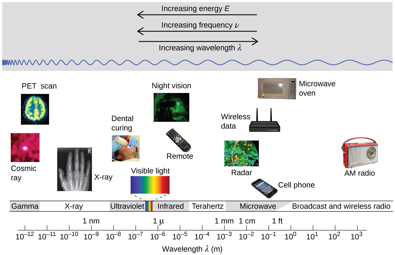
Wavelength and frequency are inversely proportional: as the wavelength increases, the frequency decreases. The inverse proportionality is illustrated in Figure 6.5. This figure also shows the electromagnetic spectrum, the range of all types of electromagnetic radiation. Each of the various colors of visible light has specific frequencies and wavelengths associated with them, and you can see that visible light makes up only a small portion of the electromagnetic spectrum. Because the technologies developed to work in various parts of the electromagnetic spectrum are different, for reasons of convenience and historical legacies, different units are typically used for different parts of the spectrum. For example, radio waves are usually specified as frequencies (typically in units of MHz), while the visible region is usually specified in wavelengths (typically in units of nm or angstroms).

.

Chemistry in Everyday Life

Wireless Communication

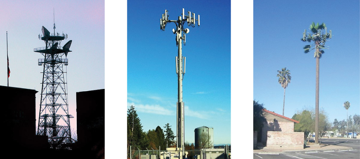
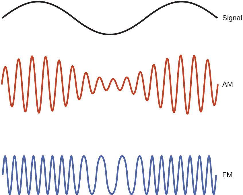
Many valuable technologies operate in the radio (3 kHz-300 GHz) frequency region of the electromagnetic spectrum (Figure 6.6). At the low frequency (low energy, long wavelength) end of this region are AM (amplitude modulation) radio signals (540-2830 kHz) that can travel long distances. FM (frequency modulation) radio signals are used at higher frequencies (87.5-108.0 MHz). In AM radio, the information is transmitted by varying the amplitude of the wave (Figure 6.7). In FM radio, by contrast, the amplitude is constant and the instantaneous frequency varies.

.

Other technologies also operate in the radio-wave portion of the electromagnetic spectrum. For example, 4G cellular telephone signals are approximately 880 MHz, while Global Positioning System (GPS) signals operate at 1.228 and 1.575 GHz, local area wireless technology (Wi-Fi) networks operate at 2.4 to 5 GHz, and highway toll sensors operate at 5.8 GHz. The frequencies associated with these applications are convenient because such waves tend not to be absorbed much by common building materials.

One particularly characteristic phenomenon of waves results when two or more waves come into contact: they interfere with each other. This phenomenon is illustrated in Figure 6.8. When the peaks (or troughs) for two waves happen to coincide, the amplitude of the wave increases. We call this increase in amplitude constructive interference. When the peaks of one wave coincide with the troughs of another wave, the amplitude of the wave decreases. We call this decrease in amplitude destructive interference.

.

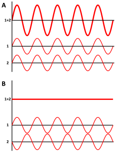
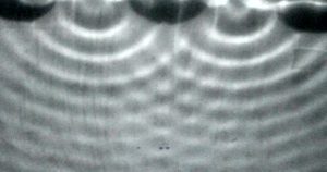
Figure 6.9 shows the interference patterns that arise when two circular waves in water interact and Figure 6.10 shows similar interference patterns that arise when light passes through narrow slits closely spaced about a wavelength apart. When the light passes through the two slits, each slit effectively acts as a new source, resulting in two closely spaced waves coming into contact at the detector (the camera in this case). The dark regions in Figure 6.10 correspond to regions of destructive interference, while the brightest regions correspond to the regions of constructive interference. The fringe patterns produced depend on the wavelength, with the fringes being more closely spaced for shorter wavelength light passing through a given set of slits. Such interference patterns cannot be explained by particles moving according to the laws of classical mechanics.

.

..

Portrait of a Chemist

Dorothy Crowfoot Hodgkin

X-rays are high energy light that exhibit wavelengths of approximately 0.01–10 nm. Since these wavelengths are comparable to the spaces between atoms in a crystalline solid, X-rays are scattered when they pass through crystals. The scattered rays undergo constructive and destructive interference that creates a specific diffraction pattern that may be measured and used to precisely determine the positions of atoms within the crystal. This phenomenon of X-ray diffraction is the basis for very powerful techniques enabling the determination of molecular structure. One of the pioneers who applied this powerful technology to important biochemical substances was Dorothy Crowfoot Hodgkin (Figure 6.11).

.

Born in Cairo, Egypt, in 1910 to British parents, Dorothy’s fascination with chemistry was fostered early in her life. At age 11 she was enrolled in a prestigious English grammar school where she was one of just two girls allowed to study chemistry. On her 16th birthday, her mother, Molly, gifted her a book on X-ray crystallography, which had a profound impact on the trajectory of her career. She studied chemistry at Oxford University, graduating with first-class honors in 1932 and directly entering Cambridge University to pursue a doctoral degree. At Cambridge, Dorothy recognized the promise of X-ray crystallography for protein structure determinations, conducting research that earned her a PhD in 1937. Over the course of a very productive career, Dr. Hodgkin was credited with determining structures for several important biomolecules, including cholesterol iodide, penicillin, and vitamin B12. In recognition of her achievements in the use of X-ray techniques to elucidate the structures of biochemical substances, she was awarded the 1964 Nobel Prize in Chemistry. In 1969, she led a team of scientists who deduced the structure of insulin, facilitating the mass production of this hormone and greatly advancing the treatment of diabetic patients worldwide. Dr. Hodgkin continued working with the international scientific community, earning numerous distinctions and awards prior to her death in 1993.

Not all waves are traveling waves. Standing waves (also known as stationary waves) remain constrained within some region of space. As we shall see, standing waves play an important role in our understanding of the electronic structure of atoms and molecules. The simplest example of a standing wave is a one-dimensional wave associated with a vibrating string that is held fixed at its two end points. Figure 6.12 shows the four lowest-energy standing waves (the fundamental wave and the lowest three harmonics) for a vibrating string at a particular amplitude. Although the string’s motion lies mostly within a plane, the wave itself is considered to be one dimensional, since it lies along the length of the string. The motion of string segments in a direction perpendicular to the string length generates the waves and so the amplitude of the waves is visible as the maximum displacement of the curves seen in Figure 6.12.

.

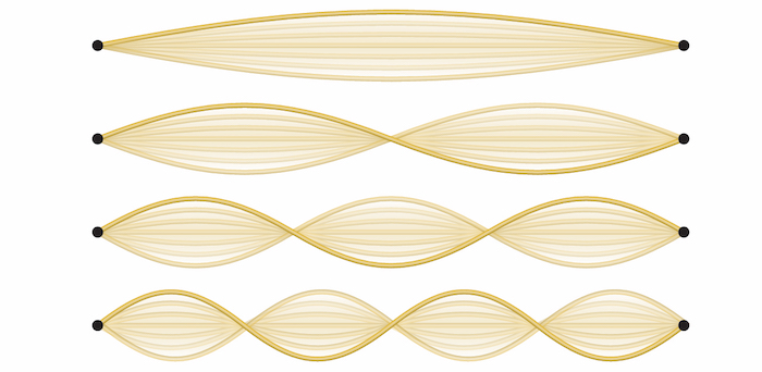
The key observation from the figure is that only those waves having an integer number, n, of half-wavelengths between the end points can form. A system with fixed end points such as this restricts the number and type of the possible waveforms. This is an example of quantization, in which only discrete values from a more general set of continuous values of some property are observed. Another important observation is that the harmonic waves (those waves displaying more than one-half wavelength) all have one or more points between the two end points that are not in motion. These special points are nodes. The energies of the standing waves with a given amplitude in a vibrating string increase with the number of half-wavelengths n. Since the number of nodes is n – 1, the energy can also be said to depend on the number of nodes, generally increasing as the number of nodes increases.

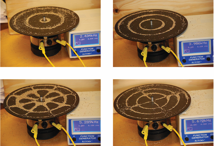
An example of two-dimensional standing waves is shown in Figure 6.13, which shows the vibrational patterns on a flat surface. Although the vibrational amplitudes cannot be seen like they could in the vibrating string, the nodes have been made visible by sprinkling the drum surface with a powder that collects on the areas of the surface that have minimal displacement. For one-dimensional standing waves, the nodes were points on the line, but for two-dimensional standing waves, the nodes are lines on the surface (for three-dimensional standing waves, the nodes are two-dimensional surfaces within the three-dimensional volume).

.

Blackbody Radiation and the Ultraviolet Catastrophe

The last few decades of the nineteenth century witnessed intense research activity in commercializing newly discovered electric lighting. This required obtaining a better understanding of the distributions of light emitted from various sources being considered. Artificial lighting is usually designed to mimic natural sunlight within the limitations of the underlying technology. Such lighting consists of a range of broadly distributed frequencies that form a continuous spectrum. Figure 6.14 shows the wavelength distribution for sunlight. The most intense radiation is in the visible region, with the intensity dropping off rapidly for shorter wavelength ultraviolet (UV) light, and more slowly for longer wavelength infrared (IR) light.

.

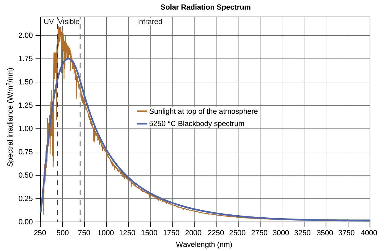
In Figure 6.14, the solar distribution is compared to a representative distribution, called a blackbody spectrum, that corresponds to a temperature of 5250°C. The blackbody spectrum matches the solar spectrum quite well. A blackbody is a convenient, ideal emitter that approximates the behavior of many materials when heated. It is “ideal” in the same sense that an ideal gas is a convenient, simple representation of real gases that works well, provided that the pressure is not too high nor the temperature too low. A good approximation of a blackbody that can be used to observe blackbody radiation is a piece of metal or rock heated to very high temperatures, like the hot lava shown in Figure 6.15.

.

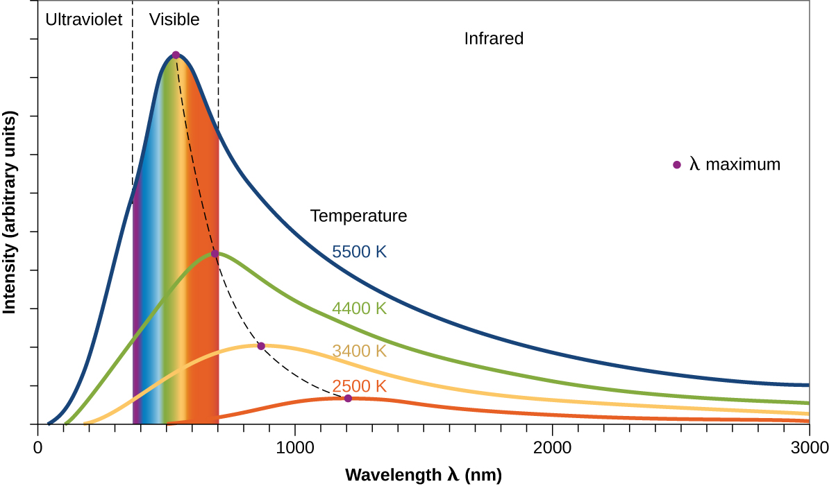
Figure 6.16 shows the resulting curves for some representative temperatures. Each distribution depends only on a single parameter: the temperature. The maxima in the blackbody curves, λ_max, shift to shorter wavelengths as the temperature increases, reflecting the observation that metals being heated to high temperatures begin to glow a darker red that becomes brighter as the temperature increases, eventually becoming white hot at very high temperatures as the intensities of all of the visible wavelengths become appreciable. This common observation was at the heart of the first paradox that showed the fundamental limitations of classical physics that we will examine.

.

Physicists derived mathematical expressions for the blackbody curves using well-accepted concepts from the theories of classical mechanics and classical electromagnetism. The theoretical expressions as functions of temperature fit the observed experimental blackbody curves well at longer wavelengths, but showed significant discrepancies at shorter wavelengths. Not only did the theoretical curves not show a peak, they absurdly showed the intensity becoming infinitely large as the wavelength became smaller, which would imply that everyday objects at room temperature should be emitting large amounts of UV light. This became known as the “ultraviolet catastrophe” because no one could find any problems with the theoretical treatment that could lead to such unrealistic short-wavelength behavior.

Finally, around 1900, Max Planck derived a theoretical expression for blackbody radiation that fit the experimental observations exactly (within experimental error). Planck developed his theoretical treatment by extending the earlier work that had been based on the premise that the atoms composing the oven vibrated at increasing frequencies (or decreasing wavelengths) as the temperature increased, with these vibrations being the source of the emitted electromagnetic radiation. But where the earlier treatments had allowed the vibrating atoms to have any energy values obtained from a continuous set of energies (perfectly reasonable, according to classical physics), Planck found that by restricting the vibrational energies to discrete values for each frequency, he could derive an expression for blackbody radiation that correctly had the intensity dropping rapidly for the short wavelengths in the UV region. Those discrete energies are represented by the following equation, where n is an integer and ν is the frequency:

The quantity h is a constant now known as Planck’s constant, in his honor. Although Planck was pleased he had resolved the blackbody radiation paradox, he was disturbed that to do so, he needed to assume the vibrating atoms required quantized energies, which he was unable to explain. The value of Planck’s constant is very small, 6.626 × 10⁻³⁴ joule seconds (J s), which helps explain why energy quantization had not been observed previously in macroscopic phenomena.

The Photoelectric Effect

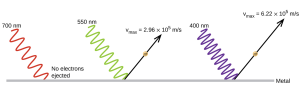
The next paradox in the classical theory to be resolved concerned the photoelectric effect (Figure 6.17). It had been observed that electrons could be ejected from the clean surface of a metal when light having a frequency greater than some threshold frequency was shone on it. Surprisingly, the kinetic energy of the ejected electrons did not depend on the brightness of the light, but increased with increasing frequency of the light. Since the electrons in the metal had a certain amount of binding energy keeping them there, the incident light needed to have more energy to free the electrons. According to classical wave theory, a wave’s energy depends on its intensity (which depends on its amplitude), not its frequency. One part of these observations was that the number of electrons ejected within in a given time period was seen to increase as the brightness increased. In 1905, Albert Einstein was able to resolve the paradox by incorporating Planck’s quantization findings into the discredited particle view of light (Einstein actually won his Nobel prize for this work, and not for his theories of relativity for which he is most famous).

.

Einstein argued that the quantized energies that Planck had postulated in his treatment of blackbody radiation could be applied to the light in the photoelectric effect so that the light striking the metal surface should not be viewed as a wave, but instead as a stream of particles (later called photons) whose energy depended on their frequency, according to Planck’s formula:

$$E=h\nu$$

or, in terms of wavelength using c = νλ

$$E=\frac{hc}{\lambda }$$

Electrons were ejected when hit by photons having sufficient energy (a frequency greater than the threshold). The greater the frequency, the greater the kinetic energy imparted to the escaping electrons by the collisions. Einstein also argued that the light intensity did not depend on the amplitude of the incoming wave, but instead corresponded to the number of photons striking the surface within a given time period. This explains why the number of ejected electrons increased with increasing brightness, since the greater the number of incoming photons, the greater the likelihood that they would collide with some of the electrons.

With Einstein’s findings, the nature of light took on a new air of mystery. Although many light phenomena could be explained either in terms of waves or particles, certain phenomena, such as the interference patterns obtained when light passed through a double slit, were completely contrary to a particle view of light, while other phenomena, such as the photoelectric effect, were completely contrary to a wave view of light. Somehow, at a deep fundamental level still not fully understood, light is both wavelike and particle-like. This is known as wave-particle duality.

Line Spectra

Another paradox within the classical electromagnetic theory that scientists in the late nineteenth century struggled with concerned the light emitted from atoms and molecules. When solids, liquids, or condensed gases are heated sufficiently, they radiate some of the excess energy as light. Photons produced in this manner have a range of energies, and thereby produce a continuous spectrum in which an unbroken series of wavelengths is present. Most of the light generated from stars (including our sun) is produced in this fashion. You can see all the visible wavelengths of light present in sunlight by using a prism to separate them. As can be seen in Figure 6.14, sunlight also contains UV light (shorter wavelengths) and IR light (longer wavelengths) that can be detected using instruments but that are invisible to the human eye. Incandescent (glowing) solids such as tungsten filaments in incandescent lights also give off light that contains all wavelengths of visible light. These continuous spectra can often be approximated by blackbody radiation curves at some appropriate temperature, such as those shown in Figure 6.16.

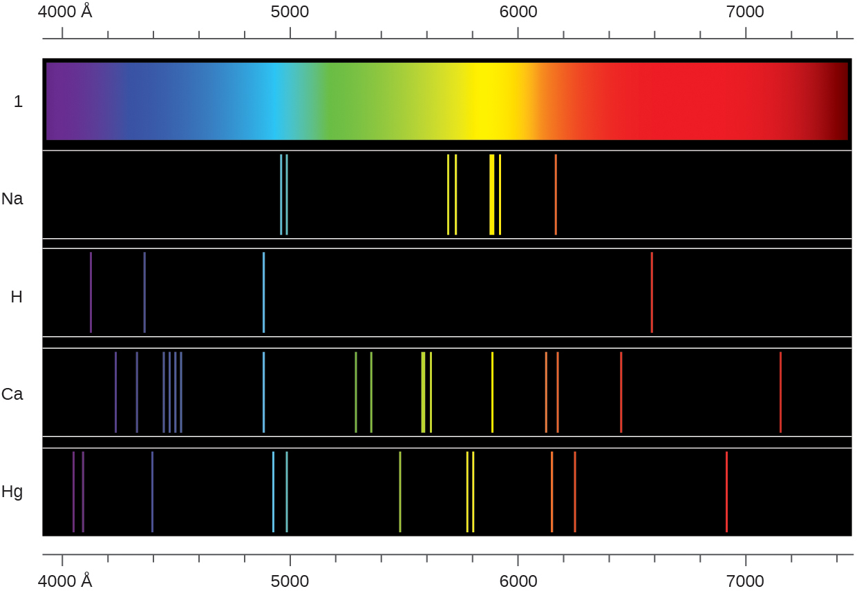
In contrast to continuous spectra, light can also occur as discrete or line spectra having very narrow line widths interspersed throughout the spectral regions such as those shown in Figure 6.19. Exciting a gas at low partial pressure using an electrical current, or heating it, will produce line spectra. Fluorescent light bulbs and neon signs operate in this way (Figure 6.18). Each element displays its own characteristic set of lines, as do molecules, although their spectra are generally much more complicated.

.

Each emission line consists of a single wavelength of light, which implies that the light emitted by a gas consists of a set of discrete energies. For example, when an electric discharge passes through a tube containing hydrogen gas at low pressure, the H₂ molecules are broken apart into separate H atoms and we see a blue-pink color. Passing the light through a prism produces a line spectrum, indicating that this light is composed of photons of four visible wavelengths, as shown in Figure 6.19.

.

The origin of discrete spectra in atoms and molecules was extremely puzzling to scientists in the late nineteenth century, since according to classical electromagnetic theory, only continuous spectra should be observed. Even more puzzling, in 1885, Johann Balmer was able to derive an empirical equation that related the four visible wavelengths of light emitted by hydrogen atoms to whole integers. That equation is the following one, in which k is a constant:

Other discrete lines for the hydrogen atom were found in the UV and IR regions. Johannes Rydberg generalized Balmer’s work and developed an empirical formula that predicted all of hydrogen’s emission lines, not just those restricted to the visible range, where n₁ and n₂ are integers, n₁ < n₂, and R_∞ is the Rydberg constant (1.097 × 10⁷ m⁻¹).

Even in the late nineteenth century, spectroscopy was a very precise science, and so the wavelengths of hydrogen were measured to very high accuracy, which implied that the Rydberg constant could be determined very precisely as well. That such a simple formula as the Rydberg formula could account for such precise measurements seemed astounding at the time, but it was the eventual explanation for emission spectra by Neils Bohr in 1913 that ultimately convinced scientists to abandon classical physics and spurred the development of modern quantum mechanics.