Main Body
6. Consumer Choices
Introduction to Consumer Choices

Chapter Overview
In this chapter, you will learn about:
- Consumption Choices
- How Changes in Income and Prices Affect Consumption Choices
- Behavioral Economics: An Alternative Framework for Consumer Choice
Bring It Home
Making Choices
The 2008–2009 Great Recession touched families around the globe. In too many countries, workers found themselves out of a job. In developed countries, unemployment compensation provided a safety net, but families still saw a marked decrease in disposable income and had to make tough spending decisions. Of course, nonessential, discretionary spending was the first to go.
Even so, during that time, there was one particular category that saw an increase in spending worldwide and an 18% uptick in the United States, specifically. You might guess that the increase occurred in grocery store spending as a result of consumers eating more meals at home, but the Bureau of Labor Statistics’ Consumer Expenditure Survey, which tracks U.S. food spending over time, showed “real total food spending by U.S. households declined five percent between 2006 and 2009.” So, it was not groceries. What product would people around the world demand more of during tough economic times, and more importantly, why? (Find out at the end of the chapter.)
That question leads us to this chapter’s topic—analyzing how consumers make choices and how changes affect those choices. For instance, do changes in prices matter more or less than changes in a consumer’s income? Can a small change in circumstances alter consumers’ perception of a product or even of their own resources? Although many choices may seem straightforward, there is often much more to consider.
Microeconomics seeks to understand the behavior of individual economic agents, such as individuals and businesses. Economists believe that we can analyze individuals’ decisions, such as what goods and services to buy, as choices they make within certain budget constraints. Generally, consumers are trying to get the most for their limited budget. In economic terms, they are trying to maximize total utility, or satisfaction, given their budget constraint.
Everyone has their personal tastes and preferences. The French say, Chacun à son goût, or “Each to his own taste.” An old Latin saying states, De gustibus non est disputandum, or “There’s no disputing about taste.” However, if people base their decisions on their own tastes and personal preferences, how can economists hope to analyze the choices consumers make?
An economic explanation for why people make different choices begins with accepting the proverbial wisdom that tastes are a matter of personal preference. However, economists also believe that the choices people make are influenced by their incomes, by the prices of the goods and services they consume, and by factors like where they live. This chapter introduces the economic theory that attempts to explain how consumers make choices about what goods and services to buy with their limited income.
The analysis in this chapter will build on the budget constraint that we introduced in the Choice in a World of Scarcity chapter. This chapter will also illustrate how economic theory provides a tool for systematically looking at the full range of possible consumption choices to predict how consumption responds to changes in prices or incomes. After reading this chapter, consult the appendix on Indifference Curves to learn more about representing utility and choice through indifference curves.
6.1 Consumption Choices
Learning Objectives
By the end of this section, you will be able to:
- Calculate total utility.
- Propose decisions that maximize utility.
- Explain marginal utility and the significance of diminishing marginal utility.
Information on the consumption choices of Americans is available from the Consumer Expenditure Survey carried out by the U.S. Bureau of Labor Statistics. Table 6.1 shows spending patterns for the average U.S. household in 2015. The first row shows income, and the second row shows that, after taxes and personal savings were subtracted, the average U.S. household spent $48,109 on consumption. The table then breaks down consumption into various categories. The average U.S. household spent roughly one third of its consumption on shelter and other housing expenses, another one third on food and vehicle expenses, and the rest on a variety of items, as shown. These patterns will vary for specific households by differing levels of family income, by geography, and by preferences.
|
Average household income before taxes |
$62,481 |
|
Average annual expenditures |
$48.109 |
|
Food at home |
$3,264 |
|
Food away from home |
$2,505 |
|
Housing |
$16,557 |
|
Apparel and services |
$1,700 |
|
Transportation |
$7,677 |
|
Healthcare |
$3,157 |
|
Entertainment |
$2,504 |
|
Education |
$1,074 |
|
Personal insurance and pensions |
$5,357 |
|
All else: alcohol, tobacco, reading, personal care, cash contributions, miscellaneous |
$3,356 |
Total Utility and Diminishing Marginal Utility
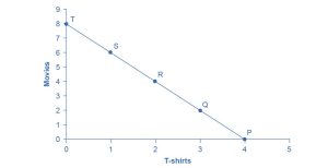
To understand how a household will make its choices, economists look at what consumers can afford, as shown in a budget constraint (or budget line), and the total utility or satisfaction derived from those choices. In a budget constraint line, the quantity of one good is on the horizontal axis, and the quantity of the other good is on the vertical axis. The budget constraint line shows the various combinations of two goods that are affordable given a consumer’s income. Consider José’s situation, shown in Figure 6.2. José likes to collect T-shirts and watch movies.
In Figure 6.2, we show the quantity of T-shirts on the horizontal axis, while we show the quantity of movies on the vertical axis. If José had unlimited income or if goods were free, then he could consume without limit. However, José, like all of us, faces a budget constraint. José has a total of $56 to spend. The price of T-shirts is $14, and the price of movies is $7. Notice that the vertical intercept of the budget constraint line is at eight movies and zero T-shirts ($56 ÷ $7 = 8). The horizontal intercept of the budget constraint is four, where José spends all of his money on T-shirts and none on movies ($56 ÷ 14 = 4). The slope of the budget constraint line is rise ÷ run, or –8 ÷ 4 = –2. The specific choices along the budget constraint line show the combinations of affordable T-shirts and movies.
José wishes to choose the combination that will provide him with the greatest utility, which is the term economists use to describe a person’s level of satisfaction or happiness with their choices.
Let’s begin with an assumption, which we will discuss in more detail later, that José can measure his utility with something called utils. (It is important to note that you cannot make comparisons between the utils of individuals. If one person gets 20 utils from a cup of coffee and another person gets 10 utils, this does not mean that the first person gets more enjoyment from the coffee than the second person or that they enjoy the coffee twice as much. The reason why is that utils are subjective to an individual. The way one person measures utils is not the same as the way someone else does.) Table 6.2 shows how José’s utility is connected with his T-shirt or movie consumption. The first column of the table shows the quantity of T-shirts consumed. The second column shows the total utility, or total amount of satisfaction, that José receives from consuming that number of T-shirts. The most common pattern of total utility, as shown in this example, is that consuming additional goods leads to greater total utility, but at a decreasing rate. The third column shows marginal utility, which is the additional utility provided by one additional unit of consumption. The equation for marginal utility is:
Notice that marginal utility diminishes as additional units are consumed, which means that each subsequent unit of a good consumed provides less additional utility. For example, the first T-shirt José picks is his favorite, and it gives him an additional 22 utils. The fourth T-shirt is just something to wear when all his other clothes are in the wash and yields only 18 additional utils. This is an example of the law of diminishing marginal utility, which holds that the additional utility decreases with each unit added. Diminishing marginal utility is another example of the more general law of diminishing returns we learned in the chapter on Choice in a World of Scarcity.
The rest of Table 6.2 shows the quantity of movies that José attends and his total and marginal utility from seeing each movie. Total utility follows the expected pattern: it increases as the number of movies that José watches rises. Marginal utility also follows the expected pattern: each additional movie brings a smaller gain in utility than the previous one. The first movie José attends is the one he wanted to see the most, and it thus provides him with the highest level of utility or satisfaction. The fifth movie he attends is just to kill time. Notice that total utility is also the sum of the marginal utilities. Read the next Work It Out feature for instructions on how to calculate total utility.
|
T-shirts (quantity) |
Total utility |
Marginal utility |
Movies (quantity) |
Total utility |
Marginal utility |
|---|---|---|---|---|---|
|
1 |
22 |
22 |
1 |
16 |
16 |
|
2 |
43 |
21 |
2 |
31 |
15 |
|
3 |
63 |
20 |
3 |
45 |
14 |
|
4 |
81 |
18 |
4 |
58 |
13 |
|
5 |
97 |
16 |
5 |
70 |
12 |
|
6 |
111 |
14 |
6 |
81 |
11 |
|
7 |
123 |
12 |
7 |
91 |
10 |
|
8 |
133 |
10 |
8 |
100 |
9 |
Table 6.3 looks at each point on the budget constraint in Figure 6.2 and adds up José’s total utility for five possible combinations of T-shirts and movies.
|
Point |
T-shirts |
Movies |
Total utility |
|
P |
4 |
0 |
81 + 0 = 81 |
|
Q |
3 |
2 |
63 + 31 = 94 |
|
R |
2 |
4 |
43 + 58 = 101 |
|
S |
1 |
6 |
22 + 81 = 103 |
|
T |
0 |
8 |
0 + 100 = 100 |
Work It Out
Calculating Total Utility
Let’s take a more detailed look at how José makes his decision.
Step 1. Observe that at point Q (for example) José consumes three T-shirts and two movies.
Step 2. Look at Table 6.2. You can see from the fourth row, second column that three T-shirts are worth 63 utils. Similarly, the second row, fifth column shows that two movies are worth 31 utils.
Step 3. From this information, you can calculate that point Q has a total utility of 94 (63 + 31).
Step 4. You can repeat the same calculations for each point on Table 6.3, using the total utility numbers shown in the last column.
For José, the highest total utility for all possible combinations of goods occurs at point S, with a total utility of 103 from consuming one T-shirt and six movies.
Choosing with Marginal Utility
Most people approach their utility-maximizing combination of choices in a step-by-step way. This approach is based on looking at the tradeoffs, measured in terms of marginal utility, of consuming less of one good and more of another.
For example, say that José starts off thinking about spending all his money on T-shirts and choosing point P, which corresponds to four T-shirts and no movies, as Figure 6.2 illustrates. José chooses this starting point randomly as he has to start somewhere. Then he considers giving up the last T-shirt, the one that provides him the least marginal utility, and using the money he saves to buy two movies instead. Table 6.4 tracks the step-by-step series of decisions José needs to make (Key: T-shirts are $14, movies are $7, and income is $56). The following Work It Out feature explains how marginal utility can affect decision making.
|
Try |
Which has |
Total utility |
Marginal gain and loss of utility, compared with previous choice |
Conclusion |
|---|---|---|---|---|
|
Choice 1: P |
4 T-shirts and 0 movies |
81 from 4 T-shirts + 0 from 0 movies = 81 |
– |
– |
|
Choice 2: Q |
3 T-shirts and 2 movies |
63 from 3 T-shirts + 31 from 0 movies = 94 |
Loss of 18 from 1 less T-shirt, but gain of 31 from 2 more movies, for a net utility gain of 13 |
Q is preferred over P |
|
Choice 3: R |
2 T-shirts and 4 movies |
43 from 2 T-shirts + 58 from 4 movies = 101 |
Loss of 20 from 1 less T-shirt, but gain of 27 from two more movies for a net utility gain of 7 |
R is preferred over Q |
|
Choice 4: S |
1 T-shirt and 6 movies |
22 from 1 T-shirt + 81 from 6 movies = 103 |
Loss of 21 from 1 less T-shirt, but gain of 23 from two more movies, for a net utility gain of 2 |
S is preferred over R |
|
Choice 5: T |
0 T-shirts and 8 movies |
0 from 0 T-shirts + 100 from 8 movies = 100 |
Loss of 22 from 1 less T-shirt, but gain of 19 from two more movies, for a net utility loss of 3 |
S is preferred over T |
Work It Out
Decision Making by Comparing Marginal Utility
José could use the following thought process (if he thought in utils) to make his decision regarding how many T-shirts and movies to purchase:
Step 1. From Table 6.2, José can see that the marginal utility of the fourth T-shirt is 18. If José gives up the fourth T-shirt, then he loses 18 utils.
Step 2. However, giving up the fourth T-shirt frees up $14 (the price of a T-shirt), allowing José to buy the first two movies (at $7 each).
Step 3. José knows that the marginal utility of the first movie is 16, and the marginal utility of the second movie is 15. Thus, if José moves from point P to point Q, he gives up 18 utils (from the T-shirt), but gains 31 utils (from the movies).
Step 4. Gaining 31 utils and losing 18 utils is a net gain of 13. This is just another way of saying that the total utility at Q (94 according to the last column in Table 6.3) is 13 more than the total utility at P (81).
Step 5. Thus, for José, it makes sense to give up the fourth T-shirt to buy two movies.
José clearly prefers point Q to point P. Now repeat this step-by-step process of decision making with marginal utilities. José thinks about giving up the third T-shirt and surrendering a marginal utility of 20 in exchange for purchasing two more movies that promise a combined marginal utility of 27. José prefers point R to point Q. What if José thinks about going beyond point R to point S? Giving up the second T-shirt means a marginal utility loss of 21, and the marginal utility gain from the fifth and sixth movies would combine to make a marginal utility gain of 23, so José prefers point S to point R.
However, if José seeks to go beyond point S to point T, he finds that the loss of marginal utility from giving up the first T-shirt is 22, while the marginal utility gain from the last two movies is only a total of 19. If José were to choose point T, his utility would fall to 100. Through these stages of thinking about marginal tradeoffs, José again concludes that point S, with one T-shirt and six movies, is the choice that will provide him with the highest level of total utility. This step-by-step approach will reach the same conclusion regardless of José’s starting point.
We can develop a more systematic way of using this approach by focusing on satisfaction per dollar. If an item costing $5 yields 10 utils, then it’s worth 2 utils per dollar spent. Marginal utility per dollar is the amount of additional utility José receives divided by the product’s price. Table 6.5 shows the marginal utility per dollar for José’s T-shirts and movies.
If José wants to maximize the utility he gets from his limited budget, he will always purchase the item with the greatest marginal utility per dollar of expenditure (assuming he can afford it with his remaining budget). José starts with no purchases. If he purchases a T-shirt, the marginal utility per dollar spent will be 1.6. If he purchases a movie, the marginal utility per dollar spent will be 2.3. Therefore, José’s first purchase will be the movie. Why? Because it gives him the highest marginal utility per dollar and is affordable. Next, José will purchase another movie. Why? Because the marginal utility of the next movie (2.14) is greater than the marginal utility of the next T-shirt (1.6). Note that when José has no T-shirts, the next one is the first one. José will continue to purchase the next good with the highest marginal utility per dollar until he exhausts his budget. He will continue purchasing movies because they give him a greater “bang for the buck” until the sixth movie, which gives the same marginal utility per dollar as the first T-shirt purchase. José has just enough in his budget to purchase both. So in total, José will purchase six movies and one T-shirt.
|
Quantity of T-shirts |
Total utility |
Marginal utility |
Marginal utility per dollar |
Quantity of movies |
Total utility |
Marginal utility |
Marginal utility per dollar |
|
1 |
22 |
22 |
22 ÷ $14 = 1.6 |
1 |
16 |
16 |
16 ÷ $7 = 2.3 |
|
2 |
43 |
21 |
21 ÷ $14 = 1.5 |
2 |
31 |
15 |
15 ÷ $7 = 2.14 |
|
3 |
63 |
20 |
20 ÷ $14 = 1.4 |
3 |
45 |
14 |
14 ÷ $7 = 2 |
|
4 |
81 |
18 |
18 ÷ $14 = 1.3 |
4 |
58 |
13 |
13 ÷ $7 = 1.9 |
|
5 |
97 |
16 |
16 ÷ $14 = 1.1 |
5 |
70 |
12 |
12 ÷ $7 = 1.7 |
|
6 |
111 |
14 |
14 ÷ $14 = 1 |
6 |
81 |
11 |
11 ÷ $7 = 1.6 |
|
7 |
123 |
12 |
12 ÷ $14 = 1.2 |
7 |
91 |
10 |
10 ÷ $7 = 1.4 |
A Rule for Maximizing Utility
This process of decision making suggests a rule to follow when maximizing utility. Because the price of T-shirts is twice as high as the price of a movie, to maximize utility, the last T-shirt that José chooses needs to provide exactly twice the marginal utility (MU) of the last movie. If the last T-shirt provides less than twice the marginal utility of the last movie, then the T-shirt is providing less “bang for the buck” (i.e., marginal utility per dollar spent) than José would receive from spending the same money on movies. If this is so, José should trade the T-shirt for more movies to increase his total utility.
If the last T-shirt provides more than twice the marginal utility of the last movie, then the T-shirt is providing more “bang for the buck,” or marginal utility per dollar, than if the money were spent on movies. As a result, José should buy more T-shirts. Notice that at José’s optimal choice of point S, the marginal utility from the first T-shirt is 22 and is exactly twice the marginal utility of the sixth movie, which is 11. At this choice, the marginal utility per dollar is the same for both goods. This is a telltale signal that José has found the point with the highest total utility.
We can write this argument as a general rule: If you always choose the item with the greatest marginal utility per dollar spent, when your budget is exhausted, the utility-maximizing choice should occur where the marginal utility per dollar spent is the same for both goods.
A sensible economizer will pay twice as much for something only if the item confers twice as much utility in the marginal comparison. Notice that the formula for Table 6.5 is:
The following Work It Out feature provides step by step guidance for this concept of utility-maximizing choices.
Work It Out
Maximizing Utility
The general rule, [latex]\frac{MU_1}{P_1}=\frac{MU_2}{P_2}[/latex], means that the last dollar spent on each good provides exactly the same marginal utility. This is the case at Point S. So:
Step 1. If we traded a dollar more of movies for a dollar more of T-shirts, the marginal utility gained from T-shirts would exactly offset the marginal utility lost from fewer movies. In other words, the net gain would be zero.
Step 2. However, products usually cost more than a dollar, so we cannot trade a dollar’s worth of movies. The best we can do is trade two movies for another T-shirt, because T-shirts cost twice as much as a movie in this example.
Step 3. If we traded two movies for one T-shirt, we would end up at R (two T-shirts and four movies).
Step 4. Choice 4 in Table 6.4 shows that if we moved to R, we would gain 21 utils from one more T-shirt, but lose 23 utils from two fewer movies, so we would end up with less total utility at R.
In short, the general rule shows us the utility-maximizing choice, which is called the consumer equilibrium.
Another way to express the general rule is to say that the ratio of the prices of the two goods should be equal to the ratio of the marginal utilities. When we divide the price of good 1 by the price of good 2, at the utility-maximizing point, this will equal the marginal utility of good 1 divided by the marginal utility of good 2.
Along the budget constraint, the total price of the two goods remains the same, so the ratio of the prices does not change. However, the marginal utility of the two goods changes with the quantities consumed. At the optimal choice of one T-shirt and six movies (S), the ratio of marginal utility to price for T-shirts (22:14) matches the ratio of marginal utility to price for movies (11:7).
Measuring Utility With Numbers
This discussion of utility began with an assumption that it is possible to place numerical values on utility, an assumption that may seem questionable. You can buy a thermometer for measuring temperature at the hardware store, but what store sells a “utilimometer” for measuring utility? Although measuring utility with numbers is a convenient assumption to clarify the explanation, the key assumption is not that an outside party can measure utility but only that individuals can decide which of two alternatives they prefer.
To understand this point, think back to the step-by-step process of finding the choice with the highest total utility by comparing the marginal utility you gain and lose from different choices along the budget constraint. As José compares each choice along his budget constraint to the previous choice, what matters is not the specific numbers that he places on his utility—or whether he uses any numbers at all—but only that he can identify which choices he prefers.
In this way, the step-by-step process of choosing the highest level of utility rather closely resembles how many people make consumption decisions. We think about what will make us the happiest. We think about what things cost. We think about buying a little more of one item and giving up a little of something else. We choose what provides us with the greatest level of satisfaction. The vocabulary used to compare the points along a budget constraint and total and marginal utility is just a set of tools for discussing this everyday process in a clear and specific manner. It is welcome news that specific utility numbers are not central to the argument, because a good utilimometer is hard to find. Do not worry. Although we cannot measure utils, by the end of the next module, we will have transformed our analysis into something we can measure—demand.
Check Your Learning
Julian is deciding how many cups of coffee to drink during his morning study session. The marginal utility he receives from each cup is shown in Table 6.6.
Table 6.6: Marginal Utility of Coffee Consumption
| Cups of coffee | Marginal utility (utils) |
| 1 | 20 |
| 2 | 16 |
| 3 | 12 |
| 4 | 6 |
Check Your Learning
(Learning Outcome: Calculate total utility.)
| Quantity | Lip gloss MU | MU per dollar | Magazine MU | MU per dollar |
| 1 | 24 | 24 ÷ 6 = 4 | 18 | 18 ÷ 3 = 6 |
| 2 | 18 | 18 ÷ 6 = 3 | 12 | 12 ÷ 3 = 4 |
| 3 | 12 | 12 ÷ 6 = 2 | 6 | 6 ÷ 3 = 2 |
Check Your Learning
(Learning Outcome: Propose decisions that maximize utility.)
Case Study: Financial Exclusion and Consumer Choices in Black-Majority Communities
In Black-majority communities across the United States, systemic financial exclusion shapes consumer choices and limits economic mobility. These communities often face reduced access to mainstream financial services, higher banking fees, and fewer opportunities for building wealth. This case study delves into the financial barriers faced by Black consumers, particularly in areas like South Side, Chicago, and explores how these barriers influence their economic decisions.
For example, a 2020 Brookings analysis found that banks in Black-majority areas are more likely to close branches and reduce services, leaving residents with limited options for saving, borrowing, and investing. This lack of access drives many Black consumers to rely on high-cost alternatives, such as payday loans with interest rates that can reach up to 400% annually or check-cashing services that charge them steep fees just to access their own money. These financial practices not only diminish disposable income but also make it difficult for consumers to build credit, save for emergencies, and invest in long-term goals like homeownership.
A McKinsey & Company report highlights the fact that Black consumers are increasingly turning to digital banking options as traditional banks continue to fail them. This shift reflects a broader dissatisfaction with mainstream financial services, which often impose high fees and lack transparency. However, although digital banking offers some relief, it does not fully address the systemic issues of financial exclusion.
In South Side, Chicago, for example, the closure of bank branches has exacerbated these challenges, forcing residents to seek out predatory lenders. This reliance on alternative financial services leads to poor financial health, limiting consumer choices and perpetuating poverty cycles. To address these disparities, there is a growing need for more equitable financial products, financial education, and policies that prioritize the needs of underserved communities. By improving access to fair banking services, communities can be empowered to make better financial decisions, ultimately leading to greater economic stability and growth.
This case study emphasizes the importance of financial inclusion in shaping consumer choices and highlights the systemic inequalities that must be addressed to improve economic outcomes for Black-majority communities.
Key Concepts and Summary
6.1 Consumption Choices
Economic analysis of household behavior is based on the assumption that people will seek the highest level of utility or satisfaction. Individuals are the only judges of their utility. In general, greater consumption of a good brings higher total utility. However, the additional utility people receive from each unit of greater consumption tends to decline in a pattern of diminishing marginal utility.
We can find the utility-maximizing choice on a consumption budget constraint in several ways. You can add up the total utility of each choice on the budget line and choose the highest total. You can select a starting point at random, compare the marginal utility gains and losses of moving to neighboring points, and eventually seek out the preferred choice. Alternatively, you can compare the ratio of the marginal utility to price of good 1 with the marginal utility to price of good 2 and apply the rule that at the optimal choice, the two ratios should be equal:
6.2 How Changes in Income and Prices Affect Consumption Choices
Learning Objectives
By the end of this section, you will be able to:
- Explain how income, prices, and preferences affect consumer choices.
- Contrast the substitution effect and the income effect.
- Utilize concepts of demand to analyze consumer choices.
- Apply utility-maximizing choices to governments and businesses.
Just as we can use utility and marginal utility to discuss making consumer choices along a budget constraint, we can also use these ideas to think about how consumer choices change when the budget constraint shifts in response to changes in income or price. Because we can use the budget constraint framework to analyze how quantities demanded change because of price movements, the budget constraint model can illustrate the underlying logic behind demand curves.
How Changes in Income Affect Consumer Choices
Let’s begin with a concrete example illustrating how changes in income level affect consumer choices. Figure 6.3 shows a budget constraint that represents Kimberly’s choice between concert tickets at $50 each and overnight stays at a bed-and-breakfast for $200 per night. Kimberly has $1,000 per year to spend between these two choices. After thinking about her total utility and marginal utility and applying the decision rule that the ratio of the marginal utilities to the prices should be equal between the two products, Kimberly chooses M, with eight concerts and three overnight stays, as her utility-maximizing choice.
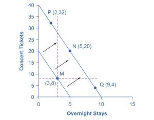
Now, assume that the income Kimberly has to spend on these two items rises to $2,000 per year, causing her budget constraint to shift out to the right. How does this rise in income alter her utility-maximizing choice? Kimberly will again consider the utility and marginal utility that she receives from concert tickets and overnight getaways, and seek her utility-maximizing choice on the new budget line, but how will her new choice relate to her original choice?
We can replace the possible choices along the new budget constraint into three groups, which are divided by the dashed horizontal and vertical lines that pass through the original choice M in the figure. All choices on the upper left of the new budget constraint that are to the left of the vertical dashed line—such as choice P, with two overnight stays and 32 concert tickets—involve less of the good on the horizontal axis but much more of the good on the vertical axis. All choices to the right of the vertical dashed line and above the horizontal dashed line—such as choice N, with five overnight getaways and 20 concert tickets—have more consumption of both goods. Finally, all choices that are to the right of the vertical dashed line but below the horizontal dashed line—such as choice Q, with four concerts and nine overnight getaways—involve less of the good on the vertical axis but much more of the good on the horizontal axis.
All of these choices are theoretically possible, depending on Kimberly’s personal preferences as expressed through the total and marginal utility she would receive from consuming these two goods. When income rises, the most common reaction is to purchase more of both goods, like choice N, which is to the upper right relative to Kimberly’s original choice M, although exactly how much more of each good will vary according to personal taste. Conversely, when income falls, the most typical reaction is to purchase less of both goods. As we defined in the chapter on Demand and Supply and again in the chapter on Elasticity, we call goods and services normal goods when a rise in income leads to a rise in the quantity consumed of that good and a fall in income leads to a fall in quantity consumed.
However, depending on Kimberly’s preferences, a rise in income could cause consumption of one good to increase while consumption of the other good declines. A choice like P means that a rise in income caused her quantity consumed of overnight stays to decline, while a choice like Q would mean that a rise in income caused her quantity of concerts to decline. Goods for which demand declines as income rises (or conversely, demand rises as income falls) are called “inferior goods.” People purchase less of an inferior good as their income rises because they can now afford the more expensive choices that they prefer. For example, a higher-income household might eat fewer hamburgers and eat more steak instead, or the household might be less likely to buy a used car and more likely to buy a new car.
How Price Changes Affect Consumer Choices
To analyze the possible effect of a change in price on consumption, let’s again use a concrete example. Figure 6.4 represents Sergei’s consumer choice between purchasing baseball bats and cameras. A price increase for baseball bats would not affect his ability to purchase cameras, but it would reduce the number of bats Sergei could afford to buy. Thus, a price increase for baseball bats, the good on the horizontal axis, causes the budget constraint to rotate inward, as if on a hinge, from the vertical axis. As in the previous section, the point labeled M represents the originally preferred point on the original budget constraint, which Sergei has chosen after contemplating his total utility and marginal utility and the tradeoffs involved along the budget constraint. In this example, the units along the horizontal and vertical axes are not numbered, so the discussion must focus on whether Sergei will consume more or less of certain goods, not on numerical amounts.
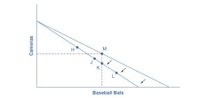
After the price increase, Sergei will make a choice along the new budget constraint. Again, we can divide his choices into three segments by the dashed vertical and horizontal lines. In the upper left portion of the new budget constraint, at a choice like H, Sergei consumes more cameras and fewer bats. In the central portion of the new budget constraint, at a choice like J, he consumes less of both goods. At the right-hand end, at a choice like L, he consumes more bats but fewer cameras.
The typical response to higher prices is for a person to choose to consume less of the product with the higher price. This occurs for two reasons, and both effects can occur simultaneously. The substitution effect occurs when a price changes and consumers have an incentive to consume less of the good with a relatively higher price and more of the good with a relatively lower price. The income effect is when a higher price means that the buying power of income has been effectively reduced (even though actual income has not changed), which leads to consumers buying less of the good (when the good is normal). In this example, the higher price for baseball bats would cause Sergei to buy fewer bats for both reasons. Exactly how much will a higher price for bats cause Sergei’s bat consumption to fall? Figure 6.4 suggests a range of possibilities. Sergei might react to a higher price for baseball bats by purchasing the same quantity of bats and cutting his camera consumption. This choice is labeled K on the new budget constraint and is located straight below M, the original choice. Alternatively, Sergei might react by dramatically reducing his bat purchases and instead buying more cameras.
The key is that it would be imprudent to assume that a change in the price of one good will only affect the consumption of that good. In our example, because Sergei purchases all his products out of the same budget, a change in the price of baseball bats can also have a range of effects, either positive or negative, on his purchases of cameras. Because Sergei purchases all his products out of the same budget, a change in the price of baseball bats can also have a range of effects, either positive or negative, on his purchases of cameras.
In short, a higher price typically causes reduced consumption of the good in question, but it can affect the consumption of other goods as well.
Check Your Learning
(Learning Outcome: Contrast the substitution effect and the income effect)
Link It Up
Read this USA Today article on the potential for Uber-style surge pricing in fast food, using Wendy’s 2025 test as a focal point: “Wendy’s plans to test dynamic pricing in 2025 through AI-powered menu boards, varying prices by time of day and demand—similar to how ride-hail apps operate.”
The Foundations of Demand Curves
Changes in the price of a good lead the budget constraint to rotate. A rotation in the budget constraint means that when individuals are seeking their highest utility, the quantity that is demanded of that good will change. In this way, the logical foundations of demand curves, which show a connection between prices and quantity demanded, are based on the underlying idea of individuals seeking utility. Figure 6.5 (a) shows a budget constraint with a choice between housing and “everything else.” (Putting “everything else” on the vertical axis can be a useful approach in some cases, especially when the focus of the analysis is on one particular good.) We label the preferred choice on the original budget constraint that provides the highest possible utility M0. The other three budget constraints represent successively higher prices for housing of P1, P2, and P3. As the budget constraint rotates in, and in, and in again, we label the utility-maximizing choices M1, M2, and M3, and the quantity demanded of housing falls from Q0 to Q1 to Q2 to Q3.
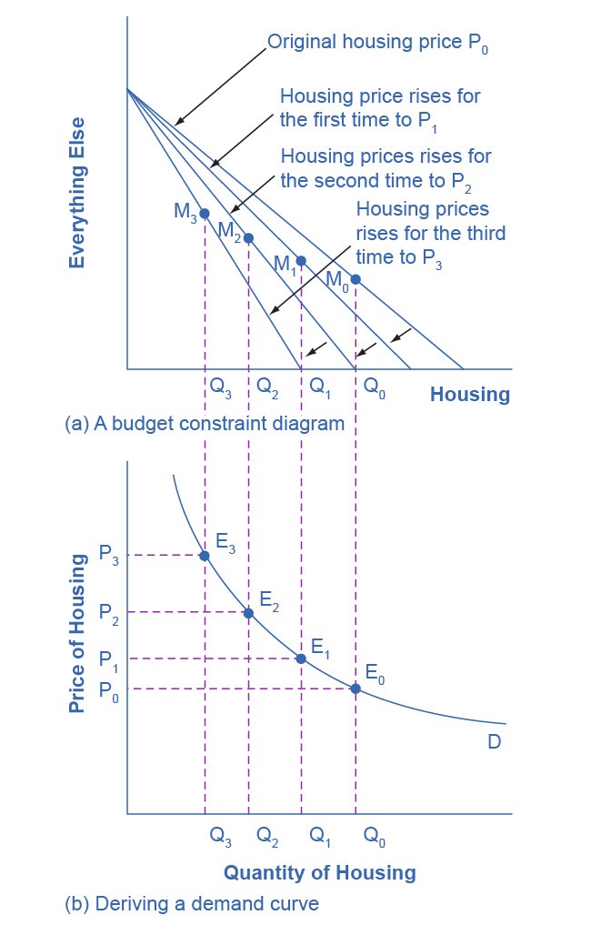
Thus, as the price of housing rises, the budget constraint rotates clockwise and the quantity consumed of housing falls, ceteris paribus (meaning, with all other things being the same). We graph this relationship—the price of housing rising from P0 to P1 to P2 to P3, while the quantity of housing demanded falls from Q0 to Q1 to Q2 to Q3—on the demand curve in Figure 6.5 (b). The vertical dashed lines stretching between the top and bottom of Figure 6.5 show that the quantity of housing demanded at each point is the same in both (a) and (b). We ultimately determine the shape of a demand curve by the underlying choices about maximizing utility subject to a budget constraint. Although economists may not be able to measure “utils,” they can certainly measure price and quantity demanded.
Applications in Government and Business
The budget constraint framework for making utility-maximizing choices offers a reminder that people can react to a change in price or income in a range of different ways. For example, in the winter months of 2005, costs for heating homes increased significantly in many parts of the country as prices for natural gas and electricity soared, due in large part to the disruption caused by Hurricanes Katrina and Rita. Some people reacted by reducing the quantity demanded of energy (e.g., by turning down the thermostats in their homes by a few degrees and wearing a heavier sweater inside). Even so, many home heating bills rose, so people adjusted their consumption in other ways, too. As you learned in the chapter on Elasticity, the short-run demand for home heating is generally inelastic. Each household cut back on what it valued least on the margin. For some, it might have meant reducing dinners at restaurants, skipping a vacation, or postponing buying a new refrigerator or a new car. Sharply higher energy prices can have effects beyond the energy market, leading to a widespread reduction in purchasing throughout the rest of the economy.
A similar issue arises when the government imposes taxes on certain products, such as gasoline, cigarettes, and alcohol. Say that a tax on alcohol leads to a higher price at the liquor store. The higher price of alcohol causes the budget constraint to pivot left, and alcoholic beverage consumption is likely to decrease. However, people may also react to the higher price of alcoholic beverages by cutting back on other purchases. For example, they might cut back on restaurant appetizers, such as chicken wings and nachos. It would be unwise to assume that the liquor industry is the only one affected by the tax on alcoholic beverages. Read the next Clear It Up to learn about how who controls the household income influences buying decisions.
The Unifying Power of the Utility-Maximizing Budget Set Framework
An interaction between prices, budget constraints, and personal preferences determines household choices. The flexible and powerful terminology related to utility maximizing gives economists a vocabulary for bringing these elements together.
Not even economists believe that people walk around mumbling about their marginal utilities before they walk into a shopping mall, accept a job, or make a deposit in a savings account. However, economists do believe that individuals seek their own satisfaction or utility and that people often decide to try a little less of one thing and a little more of another. If we accept these assumptions, then the idea of utility-maximizing households facing budget constraints becomes highly plausible.
Clear It Up
Does Who Controls Household Income Make a Difference?
In the mid-1970s, the United Kingdom made an interesting policy change in its “child allowance” policy. This program provides a fixed amount of money per child to every family, regardless of family income. Traditionally, the child allowance had been distributed to families by withholding less in taxes from the paycheck of the family wage earner, who was typically the father during this era. The new policy instead provided the child allowance as a cash payment to the mother. As a result of this change, households had the same level of income and faced the same prices in the market, but the money was more likely to be in the mother’s purse than in the father’s wallet.
Should this policy change alter household consumption patterns? Basic models of consumption decisions, of the sort that we examined in this chapter, assume that it does not matter which parent or guardian receives the money, because both seek to maximize the family’s utility as a whole. In effect, this model assumes that everyone in the family has the same makeup or has the same preferences.
There has not been extensive research on diverse family structures and guardian/parent sex and gender in relation to spending. However, the older research on families with one man parent and one woman parent indicates that gender does affect spending decisions. When the mother controls a larger share of family income, studies in the United Kingdom and in a wide variety of other countries have found that the family tends to spend more on restaurant meals, child care, and women’s clothing and less on alcohol and tobacco. As the mother controls a larger share of household resources, children’s health improves, too. These findings suggest that when providing assistance to families, in high-income countries and low-income countries alike, the monetary amount of assistance is not all that matters; rather, it also matters which family member receives the money.
The budget constraint framework serves as a constant reminder to think about the full range of effects that can arise from changes in income or price, not just effects on the one product that might seem most immediately affected.
Key Concepts and Summary
6.2 How Changes in Income and Prices Affect Consumption Choices
The budget constraint framework suggests that when income or price changes, a range of responses are possible. When income rises, households will demand a higher quantity of normal goods, but a lower quantity of inferior goods. When the price of a good rises, households will typically demand less of that good, but whether they will demand a much lower quantity or only a slightly lower quantity will depend on personal preferences. Also, a higher price for one good can lead to more or less demand for the other good.
6.3 Behavioral Economics: An Alternative Framework for Consumer Choice
Learning Objectives
By the end of this section, you will be able to:
- Evaluate the reasons for making intertemporal choices.
- Interpret an intertemporal budget constraint.
- Analyze why people in the United States tend to save such a small percentage of their income.
As we know, people sometimes make decisions that seem “irrational” and not in their own best interest. People’s decisions can seem inconsistent from one day to the next, and they may deliberately ignore ways to save money or time. The traditional economic models assume rationality, which means that people take all available information and make consistent and informed decisions that are in their best interest. (In fact, economics professors often delight in pointing out so-called “irrational behavior” to their new students each semester and present economics as a way to become more rational.)
However, a new group of economists, known as behavioral economists, argues that the traditional method omits something important: people’s state of mind. For example, one can think differently about money if one is feeling revenge, optimism, or loss. These are not necessarily irrational states of mind, but they are part of a range of emotions that can affect anyone on a given day. In addition, actions under these conditions are predictable if one better understands the underlying environment. Behavioral economics seeks to enrich our understanding of decision making by integrating the insights of psychology into economics. It does this by investigating how given dollar amounts can mean different things to individuals depending on the situation. This can lead to decisions that appear outwardly inconsistent or irrational to the outside observer.
According to this view, the way the mind works may seem inconsistent to traditional economists, but it is actually far more complex than an unemotional cost-benefit adding machine. For example, a traditional economist would say that if you lost a $10 bill today and also received an extra $10 in your paycheck, you should feel perfectly neutral. After all, –$10 + $10 = $0. You are the same financially as you were before. However, behavioral economists have conducted research that shows many people will feel some negative emotion, such as anger or frustration, after these two things happen. We tend to focus more on the loss than the gain. According to the economists Daniel Kahneman and Amos Tversky in a famous 1979 article in the journal Econometrica, when a $1 loss pains us 2.25 times more than a $1 gain helps us, we call it “loss aversion.” This insight has implications for investing, as people tend to “overplay” the stock market by reacting more to losses than to gains. This behavior looks irrational to traditional economists, but it is consistent once we better understand how the mind works, these economists argue.
Traditional economists also assume that human beings have complete self-control. However, people will buy cigarettes by the pack to keep usage down, even though buying them by the carton saves them money. Furthermore, they will purchase locks for their refrigerators and overpay on taxes to force themselves to save. In other words, we protect ourselves from our worst temptations but pay a price to do so. One way behavioral economists are responding to this is by establishing ways for people to keep themselves free of these temptations. This includes what we call “nudges” toward more rational behavior rather than mandatory regulations from the government. For example, up to 20% of new employees do not immediately enroll in retirement savings plans due to procrastination or feeling overwhelmed by the different choices. Some companies are now moving to a new system that automatically enrolls employees unless they “opt out.” Almost no one opts out of this program, and employees begin saving during their early years, which are the most critical for retirement.
Another area that seems illogical is the idea of mental accounting, or putting dollars in different mental categories where they have different values. Economists typically consider dollars to be fungible, meaning they have equal value to the individual, regardless of the situation.
You might, for instance, view the $25 you found in the street differently than the $25 you earned by working for three hours in a fast-food restaurant. You might treat the street money as “mad money” with little rational regard for getting the best value. In a sense, this is strange, because the found money is still equivalent to three hours of hard work in the restaurant. Yet the “easy come, easy go” mentality replaces the rational economizer because of the situation, or context, in which you attained the money.
In another example of mental accounting that seems inconsistent to a traditional economist, a person could carry a credit card debt of $1,000 that has a 15% yearly interest cost and simultaneously have a $2,000 savings account that earns only 2% in interest per year. This means the person pays $150 a year to the credit card company, while collecting only $40 annually in bank interest, so they lose $110 a year. That doesn’t seem wise.
The “rational” decision would be to pay off the debt, because a $1,000 savings account with $0 in debt is the equivalent net worth, and the person would now net $20 per year. Curiously, it is not uncommon for people to ignore this advice, because they will treat a loss to their savings account as greater than the benefit of paying off their credit card. In other words, they do not treat the dollars as fungible, which looks irrational to traditional economists.
Which view is right, the behavioral economists’ or the traditional view? Both have their advantages, but behavioral economists have at least tried to describe and explain behavior that economists have historically dismissed as irrational. If most of us are engaged in some “irrational behavior,” perhaps there are underlying reasons supporting this behavior.
Bring It Home
Making Choices
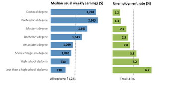
In what category did consumers worldwide increase their spending during the Great Recession? Higher education. According to the United Nations Educational, Scientific, and Cultural Organization (UNESCO), enrollment in colleges and universities rose by one third in China, almost two thirds in Saudi Arabia, nearly double in Pakistan, triple in Uganda, and 18%—or three million students—in the United States. Why were consumers willing to spend on education during lean times? Both individuals and countries view higher education as the way to prosperity. Many feel that increased earnings are a significant benefit of attending college.
U.S. Bureau of Labor Statistics data from May 2012 supports this view, as Figure 6.6 shows. The data show a positive correlation between earnings and education. The data also indicate that unemployment rates fall with higher levels of education and training.
Why spend the money to go to college during a recession? Because if you are unemployed (or underemployed, meaning you are working fewer hours than you would like), the opportunity cost of your time is low. If you’re unemployed, you don’t have to give up work hours and income by going to college.
Key Concepts and Summary
6.3 Behavioral Economics: An Alternative Framework for Consumer Choice
People regularly make decisions that seem less than rational and that contradict traditional consumer theory. This is because traditional theory ignores people’s state of mind and feelings, which can influence behavior. For example, people tend to value a dollar lost more than a dollar gained, even though the amounts are the same. Similarly, many people over-withhold on their taxes, essentially giving the government a free loan until they file their tax returns, so that they are more likely to get money back than have to pay money on their taxes.
Media Attributions
- Commencement © roanokecollege adapted by OpenStax is licensed under a CC BY (Attribution) license
- A Choice between Consumption Goods © OpenStax is licensed under a CC BY (Attribution) license
- How a Change in Income Affects Consumption Choices © OpenStax is licensed under a CC BY (Attribution) license
- How a Change in Price Affects Consumption Choices © OpenStax is licensed under a CC BY (Attribution) license
- The Foundations of a Demand Curve: An Example of Housing © OpenStax is licensed under a CC BY (Attribution) license
- Employment © U.S. Bureau of Labor Statistics is licensed under a Public Domain license
