Introduction to Unemployment

Unemployment can be a terrible and wrenching life experience with consequences only someone who has gone through it can fully understand. For unemployed individuals and their families, there is the day-to-day financial stress of not knowing when the next paycheck is coming. There are painful adjustments, like watching their savings account dwindle, selling a car and buying a cheaper one, or moving to a less expensive place to live. Even when the unemployed person finds a new job, it may pay less than the previous one. For many people, their job is an important part of their self-worth. When unemployment separates people from the workforce, it can affect their family relationships as well as their mental and physical health.

The human costs of unemployment alone would justify making a low level of unemployment an important public policy priority. However, unemployment also has economic costs for the broader society. When millions of unemployed but willing workers cannot find jobs, economic resources are unused. An economy with high unemployment is like a company operating with a functional but unused factory. The opportunity cost of unemployment is the output that the unemployed workers could have produced.

This chapter will discuss how economists define and compute the unemployment rate. It will examine the patterns of unemployment over time for the U.S. economy as a whole, for different demographic groups in the U.S. economy, and for other countries. It will then consider an economic explanation for unemployment and how it explains the patterns of unemployment and suggests public policies for reducing it.

21.1 How Economists Define and Compute the Unemployment Rate

21.2 Patterns of Unemployment

Let’s look at how unemployment rates have changed over time and how various groups of people are affected by unemployment.

The Historical U.S. Unemployment Rate

Figure 21.3 shows the historical pattern of U.S. unemployment since 1955.

As we look at this data, several patterns stand out:

• Unemployment rates fluctuate over time. During the deep recessions of the early 1980s, 2007–2009, and 2021, unemployment reached roughly 10%. For comparison, during the 1930s Great Depression, the unemployment rate reached almost 25% of the labor force.
• Unemployment rates in the late 1990s and into the mid-2000s were rather low by historical standards. The unemployment rate was below 5% from 1997 to 2000, nearly 5% during almost all of 2006 and 2007, and 5% or less from September 2015 through March 2020. The previous time unemployment had been less than 5% for 3 consecutive years was decades earlier, from 1968 to 1970.
• The unemployment rate never falls all the way to zero. It rarely falls below 3%, and it stays that low only for very short periods. (We discuss why this is the case later in this chapter.)
• The timing of rises and falls in unemployment matches fairly well with the timing of upswings and downswings in the overall economy, except that unemployment tends to lag behind changes in economic activity. This is especially true during upswings of the economy following a recession. During periods of recession and depression, unemployment is high. During periods of economic growth, unemployment tends to be lower.
• No significant upward or downward trend in unemployment rates is apparent. This point is especially worth noting because the U.S. population more than quadrupled from 76 million in 1900 to over 324 million in 2017. Moreover, a higher proportion of U.S. adults are now in the paid workforce because women have entered the paid labor force in significant numbers in recent decades. Women comprised 18% of the paid workforce in 1900 and nearly half of the paid workforce in 2021. However, despite the increased number of workers, as well as other economic events, such as globalization and the continuous invention of new technologies, the economy has provided jobs without causing any long-term upward or downward trend in unemployment rates.

Unemployment Rates by Group

Unemployment is not distributed evenly across the U.S. population. Figure 21.4 shows unemployment rates broken down by gender, age, and race/ethnicity.

The unemployment rate for women historically tended to be higher than the unemployment rate for men, perhaps reflecting the historical pattern that women were seen as “secondary” earners. By about 1980, however, the unemployment rate for women was essentially the same as that for men, as Figure 21.4 (a) shows. During the pandemic-induced recession of 2020 and in the immediate aftermath, the unemployment rate for women exceeded the unemployment rate for men. Subsequently, however, the gap has narrowed.

Younger workers tend to have higher unemployment, while middle-aged workers tend to have lower unemployment. As part of the process of matching workers and jobs, younger workers move in and out of jobs more frequently than middle-aged workers do, and this contributes to their higher unemployment rates. In addition, middle-aged workers are more likely to feel the responsibility of needing to have a job more heavily. Elderly workers have extremely low rates of unemployment because those who do not have jobs often exit the labor force by retiring and thus are not counted in the unemployment statistics. Figure 21.4 (b) shows unemployment rates for women divided by age. The pattern for men is similar.

The unemployment rate for Black Americans is substantially higher than the rate for other racial or ethnic groups, a fact that reflects, to some extent, a pattern of discrimination that has constrained Black people’s labor market opportunities. However, the gaps between unemployment rates for White, Black, and Hispanic people diminished in the 1990s, as Figure 21.4 (c) shows. In fact, unemployment rates for Black and Hispanic people were at their lowest levels in several decades in the mid-2000s before they rose during the recent Great Recession.

Finally, those with less education typically suffer higher unemployment. In November 2021, for example, the unemployment rate was 2.3% for those with a college degree, 3.7% for those with some college but not a 4-year degree, 5.2% for high school graduates with no additional degree, and 5.7% for those without a high school diploma. This pattern arises because additional education typically offers better connections to the labor market and higher demand. Facing less attractive labor market opportunities, including lower pay, low-skilled workers may be less motivated than more skilled workers to find jobs.

Breaking Down Unemployment in Other Ways

The Bureau of Labor Statistics also gives information about the reasons for unemployment and the length of time individuals have been unemployed. Table 21.2 shows the four reasons for unemployment and the percentages of the currently unemployed that fall into each category. Table 21.3 shows the length of unemployment. For both of these, the data is from November 2021.

Table 21.2 Reasons for Unemployment, November 2021 (Source: Bureau of Labor Statistics) 

Reason	Percentage
New entrants	6.5%
Re-entrants	31.8%
Job leavers	12.5%
Job losers: temporary	11.8%
Job losers: nontemporary	37.3%

Table 21.3 Length of Unemployment, November 2021

Length of time	Percentage
Under 5 weeks	22.3%
5 to 14 weeks	22.3%
15 to 26 weeks	17.6%
Over 27 weeks	37.7%

International Unemployment Comparisons

From an international perspective, the U.S. unemployment rate typically looks a little better than average. Table 21.4 compares unemployment rates for 1991, 1996, 2001, 2006 (just before the Great Recession), and 2019 (just before the pandemic-induced recession) from several other high-income countries.

Table 21.4 International Comparisons of Unemployment Rates

Country	1991	1996	2001	2006	2019
United States	6.8%	5.4%	4.8%	4.4%	3.7%
Canada	9.8%	8.8%	6.4%	6.2%	5.7%
Japan	2.1%	3.4%	5.1%	4.5%	2.4%
France	9.5%	12.5%	8.7%	10.1%	8.5%
Germany	5.6%	9.0%	8.9%	9.8%	3.1%
Italy	6.9%	11.7%	9.6%	7.8%	10.0%
Sweden	3.1%	9.9%	5.0%	5.2%	7.0%
United Kingdom	8.8%	8.1%	5.1%	5.5%	3.9%

However, we need to treat cross-country comparisons of unemployment rates with care, because each country has slightly different definitions of unemployment and survey tools for measuring unemployment, as well as different labor markets. For example, Japan’s unemployment rates appear quite low, but Japan’s economy has been mired in slow growth and recessions since the late 1980s, and Japan’s unemployment rate probably paints too rosy a picture of its labor market. In Japan, workers who lose their jobs are often quick to exit the labor force and stop looking for a new job, in which case they are not counted as unemployed. In addition, Japanese firms are often quite reluctant to fire workers. As a result, firms have substantial numbers of workers who work reduced hours or who are officially employed, but do very little. We can view this pattern as an unusual way for society to provide support to the unemployed, rather than as a sign of a healthy economy.

Comparing unemployment rates in the United States and other high-income economies with unemployment rates in Latin America, Africa, Eastern Europe, and Asia is very difficult. One reason for this is that the statistical agencies in many poorer countries lack the resources and technical capabilities of the U.S. Census Bureau. However, a more difficult problem with international comparisons is that in many low-income countries, most workers are not involved in the labor market through an employer who pays them regularly. Instead, workers in these countries are engaged in short-term work, subsistence activities, and barter. Moreover, the effect of unemployment is very different in high-income and low-income countries. Unemployed workers in developed economies have access to various government programs, such as unemployment insurance, welfare, and food stamps. Such programs may barely exist in poorer countries. Although unemployment is a serious problem in many low-income countries, it manifests itself in a different way than it does in high-income countries.

21.3 What Causes Changes in Unemployment Over the Short Run

We have seen that unemployment varies across times and places. What causes changes in unemployment? There are different answers in the short run and the long run. Let’s look at the short run first.

Cyclical Unemployment

Let’s make the plausible assumption that in the short run (e.g., from a few months to a few years), the quantity of hours that the average person is willing to work for a given wage does not change much, so the labor supply curve does not shift much. In addition, make the standard ceteris paribus assumption that there is no substantial short-term change in the age structure of the labor force, institutions and laws affecting the labor market, or other possibly relevant factors.

One primary determinant of firms’ demand for labor is how they perceive the state of the macro economy. If firms believe that business is expanding, then they will desire to hire a greater quantity of labor at any given wage, and the labor demand curve will shift to the right. Conversely, if firms perceive that the economy is slowing down or entering a recession, then they will wish to hire a lower quantity of labor at any given wage, and the labor demand curve will shift to the left. Economists call the variation in unemployment that the economy causes while moving from expansion to recession or from recession to expansion (i.e., the business cycle) cyclical unemployment.

From the standpoint of the supply-and-demand model of competitive and flexible labor markets, unemployment represents something of a puzzle. In the supply-and-demand model of a labor market, as Figure 21.5 illustrates, the labor market should move toward an equilibrium wage and quantity. At the equilibrium wage (We), the equilibrium quantity (Qe) of labor supplied by workers should be equal to the quantity of labor demanded by employers.

One possibility to consider is that people who are unemployed are those who are not willing to work at the current equilibrium wage, say $10 an hour, but would be willing to work at a higher wage, such as $20 per hour. The monthly CPS would count these people as unemployed because they say they are ready and looking for work (at $20 per hour). However, from an economist’s perspective, these people are choosing to be unemployed.

Although a few people are likely unemployed because of unrealistic expectations about wages, they do not represent the majority of the unemployed. Instead, unemployed people often have friends or acquaintances of similar skill levels who are employed, and the unemployed would be willing to work at jobs and for wages similar to what those other people are receiving. However, the employers of their friends and acquaintances do not seem to be hiring. In other words, these people are involuntarily unemployed. What causes involuntary unemployment?

Why Wages Might Be Sticky Downward

If a labor market model with flexible wages does not describe unemployment very well—because it predicts that anyone willing to work at the going wage can always find a job—then it may prove useful to consider economic models in which wages are not flexible or adjust only very slowly. In particular, even though wage increases may occur with relative ease, wage decreases are few and far between.

One set of reasons why wages may be “sticky downward,” as economists put it, involves economic laws and institutions. For low-skilled workers receiving minimum wage, it is illegal to reduce their wages. For union workers operating under a multiyear contract with a company, wage cuts might violate the contract and create a labor dispute or a strike. However, minimum wages and union contracts do not explain why wages would be sticky downward for the U.S. economy as a whole. After all, out of the 73.3 million or so employed workers in the U.S. economy who earn wages by the hour, only about 1.1 million—less than 2% of the total—do not receive compensation above the minimum wage. Similarly, labor unions represent only about 12% of U.S. wage and salary workers. In other high-income countries, more workers may have their wages determined by unions, or the minimum wage may be set at a level that applies to a larger share of workers. However, for the United States, these two factors combined affect only about 15% or less of the labor force.

Economists looking for reasons why wages might be sticky downward have focused on factors that may characterize most labor relationships in the economy, not just a few. Many have proposed a number of different theories, but they share a common tone.

One argument is that even employees who are not union members often work under an implicit contract, which is that the employer will try to keep wages from falling when the economy is weak or the business is having trouble, and the employee will not expect huge salary increases when the economy or the business is strong. This wage-setting behavior acts like a form of insurance: the employee has some protection against wage declines in bad times, but they pay for that protection with lower wages in good times. This sort of implicit contract means that firms will be hesitant to cut wages, lest workers feel betrayed and put in less effort or even leave the firm.

Efficiency wage theory argues that workers’ productivity depends on their pay, and so employers will often find it worthwhile to pay their employees somewhat more than market conditions might dictate. One reason for this is that employees who receive better pay than others will be more productive because they recognize that if they were to lose their current jobs, they would suffer a decline in salary. As a result, they are motivated to work harder and to stay with their current employer. In addition, employers know that it is costly and time-consuming to hire and train new employees, so they would prefer to pay workers a little extra now rather than lose them and have to hire and train new workers. Thus, by avoiding wage cuts, the employer minimizes the costs of training and hiring new workers and reaps the benefits of motivated employees.

The adverse selection of wage cuts argument points out that if an employer reacts to poor business conditions by reducing wages for all workers, then the best workers, who have the best employment alternatives at other firms, will be the most likely to leave. The least attractive workers, who have fewer employment alternatives, are more likely to stay. Consequently, firms are more likely to choose which workers should depart through layoffs and firings than to trim wages across the board. Occasionally, companies that are experiencing difficult times can persuade workers to take a pay cut for the short term and still retain most of their workers. However, it is far more typical for companies to lay off some workers than to cut wages for everyone.

The insider-outsider model of the labor force, in simple terms, argues that those already working for firms are “insiders,” while new employees, at least for a time, are “outsiders.” A firm depends on its insiders to keep the organization running smoothly, to be familiar with routine procedures, and to train new employees. However, cutting wages will alienate the insiders and damage the firm’s productivity and prospects.

Finally, the relative wage coordination argument points out that even if most workers were hypothetically willing to see a decline in their wages in bad economic times as long as everyone else also experiences such a decline, there is no obvious way for a decentralized economy to implement such a plan. Instead, workers confronted with the possibility of a wage cut will worry that other workers will not have such a wage cut, and so a wage cut means being worse off both in absolute terms and relative terms. As a result, workers fight hard against wage cuts.

These theories about why wages tend not to move downward differ in their logic and their implications, and figuring out the strengths and weaknesses of each theory is an ongoing subject of research and controversy among economists. They all tend to imply that wages will decline only very slowly, if at all, even when the economy or a business is having tough times. When wages are inflexible and unlikely to fall, then either short-run or long-run unemployment can result. Figure 21.6 illustrates this.

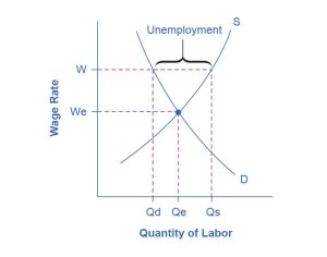
Figure 21.7 shows the interaction between shifts in labor demand and wages that are sticky downward. Figure 21.7 (a) illustrates the situation in which the demand for labor shifts to the right from D₀ to D₁. In this case, the equilibrium wage rises from W₀ to W₁, and the equilibrium quantity of labor hired increases from Q₀ to Q₁. It does not hurt employee morale at all for wages to rise.

Figure 21.7 (b) shows the situation in which the demand for labor shifts to the left, from D₀ to D₁, as it would tend to do in a recession. Because wages are sticky downward, they do not adjust toward what would have been the new equilibrium wage (W₁), at least not in the short run. Instead, after the shift in the labor demand curve, the same quantity of workers is willing to work at that wage as before. However, the quantity of workers demanded at that wage has declined from the original equilibrium (Q₀) to Q₂. The gap between the original equilibrium quantity (Q₀) and the new quantity demanded of labor (Q₂) represents workers who would be willing to work at the going wage but cannot find jobs. The gap represents the economic meaning of unemployment.

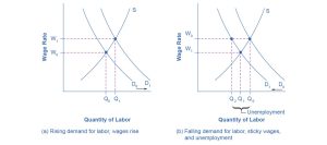
This analysis helps to explain the connection that we noted earlier: that unemployment tends to rise in recessions and to decline during expansions. The overall state of the economy shifts the labor demand curve and, combined with wages that are sticky downward, unemployment changes. The rise in unemployment that occurs because of a recession is cyclical unemployment.

Check Your Learning

 

21.4 What Causes Changes in Unemployment Over the Long Run

Cyclical unemployment explains why unemployment rises during a recession and falls during an economic expansion, but what explains the level of unemployment that remains even in good economic times? Why is the unemployment rate never zero? Even when the U.S. economy is growing strongly, the unemployment rate only rarely dips as low as 4%. Moreover, the discussion earlier in this chapter pointed out that the unemployment rates in many European countries, such as Italy, France, and Germany, have often been remarkably high at various times in the last few decades. Why does some level of unemployment persist even when economies are growing strongly? Why are unemployment rates continually higher in certain economies, through good economic years and bad? Economists call the remaining level of unemployment that occurs even when the economy is healthy the natural rate of unemployment.

The Long Run: The Natural Rate of Unemployment

The natural rate of unemployment is not “natural” in the sense that water freezes at 32 degrees Fahrenheit or boils at 212 degrees Fahrenheit. It is not a physical and unchanging law of nature. Instead, it is only the “natural” rate because it is the unemployment rate that would result from the combination of economic, social, and political factors that exist at a given time, assuming the economy was neither booming nor in recession. These forces include the usual pattern of companies expanding and contracting their workforces in a dynamic economy, social and economic forces that affect the labor market, or public policies that affect either the eagerness of people to work or the willingness of businesses to hire. Let’s discuss these factors in more detail.

Frictional Unemployment

In a market economy, some companies are always going broke for a variety of reasons, such as issues with old technology, poor management, good management that happened to make bad decisions, shifts in consumer tastes, a large customer who went broke, and tough domestic or foreign competitors. Conversely, other companies will be doing very well for just the opposite reasons and looking to hire more employees. In a perfect world, all of those who lost jobs would immediately find new ones. However, in the real world, even if the number of job seekers is equal to the number of job vacancies, it takes time to find out about new jobs, go through the interview process, and decide if the new job is a good match. Economists call the unemployment that occurs while workers move between jobs frictional unemployment. Frictional unemployment is not inherently a bad thing. It takes time to match those looking for employment with the correct job openings. For individuals and companies to be successful and productive, you want people to find the job for which they are best suited, not just the first job offered.

In the mid-2000s, before the 2008–2009 recession, it was true that about 7% of U.S. workers saw their jobs disappear in any 3-month period. However, in periods of economic growth, these destroyed jobs are counterbalanced for the economy as a whole by a larger number of jobs created. In 2019, for example, there were typically about 6 million unemployed people at any given time in the U.S. economy. Even though about two thirds of those unemployed people found a job in 14 or fewer weeks, the unemployment rate did not change much during the year because those who found new jobs were largely offset by others who lost jobs.

Of course, it would be preferable if people who were losing jobs could immediately and easily move into newly created jobs, but as we’ve discussed, that is not realistic. Someone who is laid off by a textile mill in South Carolina cannot turn around and immediately start working for a textile mill in California. Instead, the adjustment process happens in ripples. Some people find new jobs near their old ones, while others find that they must move to new locations. Some people can do a very similar job with a different company, while others must start new career paths. Some people may be near retirement and decide to look only for part-time work, while others want an employer that offers a long-term career path. The frictional unemployment that results from people moving between jobs in a dynamic economy may account for 1–2% of total unemployment.

The level of frictional unemployment will depend on how easy it is for workers to learn about alternative jobs, which may reflect the ease of communication about job prospects in the economy. The extent of frictional unemployment will also depend to some extent on how willing people are to move to new areas to find jobs, which in turn may depend on history and culture.

Frictional unemployment and the natural rate of unemployment also seem to depend on the age distribution of the population. Figure 21.4 (b) shows that unemployment rates are typically lower for people between 25 and 54 years of age and for people aged 55 and over than they are for those who are younger. “Prime-age workers,” as those in the 25–54 age bracket are sometimes called, are typically at a place in their lives when they want to have a job and income arriving at all times. In addition, older workers who lose jobs may prefer to opt for retirement. By contrast, it is likely that a relatively high proportion of those who are under 25 will be trying out jobs and life options, and this leads to greater job mobility and hence higher frictional unemployment. Thus, a society with a relatively high proportion of young workers, such as the United States when baby boomers began entering the labor market in the mid-1960s, will tend to have a higher unemployment rate than a society with a higher proportion of older workers.

Structural Unemployment

Another factor that influences the natural rate of unemployment is structural unemployment. The structurally unemployed are individuals who have no jobs because they lack skills valued by the labor market, either because demand has shifted away from the skills they do have or because they never learned any skills. An example of the former would be the unemployment among aerospace engineers after the U.S. space program downsized in the 1970s. An example of the latter would be high school dropouts.

Some people worry that technology causes structural unemployment. In the past, new technologies have put lower-skilled employees out of work. At the same time, they create demand for higher-skilled workers to use the new technologies. Education seems to be the key to minimizing the amount of structural unemployment. Individuals who have degrees can be retrained if they become structurally unemployed. For people with no skills and little education, options are more limited.

Check Your Learning

(Learning Outcome: Distinguish between frictional and structural unemployment.)

Natural Unemployment and Potential Real GDP

The natural unemployment rate is related to two other important concepts: full employment and potential real GDP. Economists consider the economy to be at full employment when the actual unemployment rate is equal to the natural unemployment rate. When the economy is at full employment, real GDP is equal to potential real GDP. In contrast, when the economy is below full employment, the unemployment rate is greater than the natural unemployment rate, and real GDP is less than potential real GDP. Finally, when the economy is above full employment, the unemployment rate is less than the natural unemployment rate, and real GDP is greater than potential real GDP. Operating above potential real GDP is only possible for a short while because it is analogous to all workers working overtime.

Productivity Shifts and the Natural Rate of Unemployment

Unexpected shifts in productivity can have a powerful effect on the natural rate of unemployment. Over time, workers’ productivity determines the level of wages in an economy. After all, if a business paid workers more than could be justified by their productivity, the business would ultimately lose money and go bankrupt. Conversely, if a business tries to pay workers less than their productivity, then, in a competitive labor market, other businesses will find it worthwhile to hire away those workers and pay them more.

However, adjustments of wages to productivity levels will not happen quickly or smoothly. Employers typically review wages only once or twice a year. In many modern jobs, it is difficult to measure productivity at the individual level. For example, how precisely would one measure the quantity produced by an accountant who is one of many people working in the tax department of a large corporation? Because productivity is difficult to observe, employers often determine wage increases based on recent experience with productivity. If productivity has been rising at 2% per year, then wages will rise at that level, as well. However, when productivity changes unexpectedly, it can affect the natural rate of unemployment for a time.

The U.S. economy in the 1970s and 1990s provides two vivid examples of this process. In the 1970s, productivity growth slowed down unexpectedly (as we discussed in Economic Growth). For example, the output per hour of U.S. workers in the business sector increased at an annual rate of 3.3% per year from 1960 to 1973, but it only increased by an annual rate of 0.8% from 1973 to 1982. Figure 21.8 (a) illustrates how the demand for labor—that is, the quantity of labor that businesses are willing to hire at any given wage—has been shifting out a little each year (from D₀ to D₁ to D₂) due to rising productivity. As a result, equilibrium wages have been rising each year from W₀ to W₁ to W₂. However, when productivity unexpectedly slows down, the pattern of wage increases does not adjust right away. Wages keep rising each year from W₂ to W₃ to W₄, but the demand for labor is no longer shifting up. A gap opens where the quantity of labor supplied at wage level W₄ is greater than the quantity demanded. The natural rate of unemployment rises. In the aftermath of this unexpectedly low productivity in the 1970s, the national unemployment rate did not fall below 7% from May 1980 until 1986. Over time, the rise in wages will adjust to match the slower gains in productivity, and the unemployment rate will ease back down, but this process may take years.

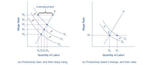
The late 1990s provide an opposite example: instead of the surprise decline in productivity that occurred in the 1970s, productivity unexpectedly rose in the mid-1990s. The annual growth rate of real output per hour of labor increased from 1.7% from 1980–1995 to an annual rate of 2.6% from 1995–2001. Let’s simplify the situation a bit so that the economic lesson of the story is easier to see graphically. Say that productivity was not increasing at all in earlier years, so the intersection of the labor market was at point E in Figure 21.8 (b), where the demand curve for labor (D₀) intersects the supply curve for labor. As a result, real wages were not increasing. Now, productivity jumps upward, which shifts the demand for labor to the right, from D₀ to D₁. However, wages are still set according to the earlier expectations of no productivity growth, so wages do not rise for a time. The result is that at the prevailing wage level (W), the quantity of labor demanded (Qd) will, for a time, exceed the quantity of labor supplied (Qs), and unemployment will be very low—below the natural level of unemployment—for a time. This pattern of unexpectedly high productivity helps to explain why the unemployment rate stayed below 4.5%, which is quite a low level by historical standards, from 1998 until after the U.S. economy entered a recession in 2001.

Levels of unemployment will tend to be somewhat higher on average when productivity is unexpectedly low. Conversely, they will tend to be somewhat lower on average when productivity is unexpectedly high. However, wages do adjust over time to reflect productivity levels.

Public Policy and the Natural Rate of Unemployment

Public policy can also have a powerful effect on the natural rate of unemployment. On the supply side of the labor market, public policies to assist the unemployed can affect how eager people are to find work. For example, if a worker who loses a job is guaranteed a generous package of unemployment insurance, welfare benefits, food stamps, and government medical benefits, then the opportunity cost of unemployment is lower, and that worker will be less eager to seek a new job.

What seems to matter most is not the amount of these benefits, but how long they last. A society that provides generous help to the unemployed that cuts off after 6 months may provide less of an incentive for unemployment than a society that provides less generous help that lasts for several years. Conversely, government assistance for job search or retraining can sometimes encourage people to go back to work sooner. See the Clear it Up to learn how the United States handles unemployment insurance.

On the demand side of the labor market, government rules, social institutions, and the presence of unions can affect the willingness of firms to hire. For example, if a government makes it hard for businesses to start up or to expand by wrapping them in bureaucratic red tape, then businesses will become more discouraged about hiring. Government regulations can make it harder to start a business by requiring that a new business obtain many permits and pay many fees, or by restricting the types and quality of products that a company can sell. Other government regulations, such as zoning laws, may limit where companies can conduct business or whether businesses are allowed to be open during the evening or on Sundays.

Whatever rationales may be offered for such laws in terms of social value—such as the value some Muslim people place on not working on Friday, or some Jewish people place on not working on Saturday, or some Christian people place on not working on Sunday—these kinds of restrictions create a difference between some willing workers and other willing employers, and thus contribute to a higher natural rate of unemployment. Similarly, if the government makes it difficult to fire or lay off workers, businesses may react by trying not to hire more workers than strictly necessary because laying these workers off would be costly and difficult. High minimum wages may discourage businesses from hiring low-skill workers. Government rules may encourage and support powerful unions, which can then push up wages for union workers, but at a cost of discouraging businesses from hiring those workers.

The Natural Rate of Unemployment in Recent Years

The underlying economic, social, and political factors that determine the natural rate of unemployment can change over time, which means that the natural rate of unemployment can change over time, too.

Economists’ estimates of the natural rate of unemployment in the U.S. economy in the early 2000s run from about 4.5% to 5.5%. This is a lower estimate than was given earlier. We will outline three of the common reasons why economists propose this change.

First, the internet has provided a remarkable new tool through which job seekers can find out about jobs at different companies and can make contact with relative ease. An internet search is far easier than trying to find a list of local employers, hunting down phone numbers for all of their human resources departments, and requesting a list of jobs and application forms. Social networking sites, such as LinkedIn, have also changed how people find work.

In addition, the growth of the temporary worker industry has probably helped to reduce the natural rate of unemployment. In the early 1980s, only about 0.5% of all workers held jobs through temp agencies. By the early 2000s, the figure had risen above 2%. Temp agencies can provide jobs for workers while they are looking for permanent work. They can also serve as a clearinghouse, helping workers find out about jobs with certain employers and try them out without long-term commitment from either side. For many workers, a temp job is a stepping-stone to a permanent job that they might not have heard about or obtained any other way, so the growth of temp jobs will also tend to reduce frictional unemployment.

The aging of the “baby boom generation”—the especially large generation of Americans born between 1946 and 1964—meant that the proportion of young workers in the economy was relatively high as the boomers entered the labor market in the late 1960s and 1970s, but that proportion is relatively low today. As we noted earlier, middle-aged and older workers are far more likely to experience low unemployment than younger workers, a factor that tends to reduce the natural rate of unemployment as the baby boomers age.

The combined result of these factors is that the natural rate of unemployment was, on average, lower in the 1990s and the early 2000s than in the 1980s. The 2008–2009 Great Recession pushed monthly unemployment rates up to 10% in late 2009. However, even at that time, the Congressional Budget Office was forecasting that by 2015, unemployment rates would fall back to about 5%. During the first 2 months of 2020, the unemployment rate held steady at 3.5%. As of the first quarter of 2022, the Congressional Budget Office estimates the natural rate to be 4.6%.

The Natural Rate of Unemployment in Europe

By the standards of other high-income economies, the natural rate of unemployment in the U.S. economy appears relatively low. Through good economic years and bad, many European economies have had unemployment rates hovering near 10%, or even higher, since the 1970s. European rates of unemployment have been higher not because recessions in Europe have been deeper, but rather because the conditions underlying supply and demand for labor have been different in Europe in a way that has created a much higher natural rate of unemployment.

Many European countries have a combination of generous welfare and unemployment benefits and nests of rules that impose additional costs on businesses when they hire. In addition, many countries have laws that require firms to give workers months of notice before laying them off and to provide substantial severance or retraining packages after laying them off. The legally required notice before laying off a worker can be more than 3 months in Spain, Germany, Denmark, and Belgium, and the legally required severance package can be as high as a year’s salary or more in Austria, Spain, Portugal, Italy, and Greece. Such laws discourage laying off or firing current workers. However, when companies know that it will be difficult to fire or lay off workers, they also become hesitant to hire workers in the first place.

We can attribute the typically higher levels of unemployment in many European countries in recent years, which have prevailed even when economies are growing at a solid pace, to the fact that the sorts of laws and regulations that lead to a high natural rate of unemployment are much more prevalent in Europe than in the United States.

A Preview of Policies to Fight Unemployment

The Government Budgets and Fiscal Policy and Macroeconomic Policy Around the World chapters provide a detailed discussion of how to fight unemployment, enabling us to discuss these policies in the context of the full array of macroeconomic goals and frameworks for analysis. However, even at this preliminary stage, it is useful to preview the main issues concerning policies to fight unemployment.

The remedy for unemployment will depend on the diagnosis. Cyclical unemployment is a short-term problem that is caused by the economy being in a recession. Thus, the preferred solution will be to avoid or minimize recessions. As Government Budgets and Fiscal Policy discusses, governments can enact this policy by stimulating the overall buying power in the economy so that firms perceive that sales and profits are possible, which makes them eager to hire.

Dealing with the natural rate of unemployment is trickier. In a market-oriented economy, firms will hire and fire workers. Governments cannot control this. Furthermore, the evolving age structure of the economy’s population and unexpected shifts in productivity are beyond a government’s control and will affect the natural rate of unemployment for a time. However, as the example of high ongoing unemployment rates for many European countries illustrates, government policy clearly can affect the natural rate of unemployment that persists even when GDP is growing.

When a government enacts policies that affect workers or employers, it must examine how these policies will affect the information and incentives employees and employers have to find one another. For example, the government may have a role to play in helping some of the unemployed with job searches. Governments may need to rethink the design of their programs that offer assistance to unemployed workers and protections to employed workers so that they will not unduly discourage the supply of labor. Similarly, governments may need to reassess rules that make it difficult for businesses to begin or to expand so that they will not unduly discourage the demand for labor. The message is not that governments should repeal all laws affecting labor markets, but rather that a society that cares about unemployment will need to consider the tradeoffs involved when they enact such laws.

Check Your Learning

(Learning Outcome: Propose ways to combat unemployment.)