Introduction to the Macroeconomic Perspective

Macroeconomics focuses on the economy as a whole (or on whole economies as they interact). What causes recessions? What makes unemployment stay high when recessions are supposed to be over? Why do some countries grow faster than others? Why do some countries have higher standards of living than others? These are all questions that macroeconomics addresses. Macroeconomics involves adding up the economic activity of all households and all businesses in all markets to obtain the overall demand and supply in the economy. However, when we do that, something curious happens. It is not unusual that what results at the macro level is different from the sum of the microeconomic parts. What seems sensible from a microeconomic point of view can have unexpected or counterproductive results at the macroeconomic level. Imagine that you are sitting at an event with a large audience, like a live concert or a basketball game. A few people decide that they want a better view, and so they stand up. However, when these people stand up, they block the view for other people, and the others need to stand up as well if they wish to see. Eventually, nearly everyone is standing up, and as a result, no one can see much better than before. The rational decision of some individuals at the micro level—to stand up for a better view—ended up as self-defeating at the macro level. This is not macroeconomics, but it is an apt analogy.

Macroeconomics is a rather massive subject. How are we going to tackle it? Figure 19.2 illustrates the structure we will use. We will study macroeconomics from three different perspectives:

1. What are the macroeconomic goals? (Macroeconomics as a discipline does not have goals, but we do have goals for the macro economy.)
2. What are the frameworks economists can use to analyze the macroeconomy?
3. Finally, what are the policy tools governments can use to manage the macroeconomy?

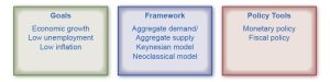
Goals

In thinking about the macroeconomy’s overall health, it is useful to consider three primary goals: economic growth, low unemployment, and low inflation.

Economic growth ultimately determines the prevailing standard of living in a country. Economists measure growth by the percentage change in real (inflation-adjusted) gross domestic product. A growth rate of more than 3% is considered good.

Unemployment, as measured by the unemployment rate, is the percentage of people in the labor force who do not have a job. When people lack jobs, the economy is wasting a precious resource-labor, and the result is lower goods and services produced. Unemployment, however, is more than a statistic—it represents people’s livelihoods. While measured unemployment is unlikely to ever be zero, economists consider a measured unemployment rate of 5% or less low (good).

Inflation is a sustained increase in the overall level of prices, and is measured by the consumer price index. If many people face a situation where the prices that they pay for food, shelter, and healthcare are rising much faster than the wages they receive for their labor, there will be widespread unhappiness as their standard of living declines. For that reason, low inflation—an inflation rate of 1–2%—is a major goal.

Frameworks

As you learn in the micro part of this book, principal tools that economists use are theories and models (see Welcome to Economics! for more on this). In microeconomics, we used the theories of supply and demand. In macroeconomics, we use the theories of aggregate demand (AD) and aggregate supply (AS). This book presents two perspectives on macroeconomics: the Neoclassical perspective and the Keynesian perspective, each of which has its own version of AD and AS. Between the two perspectives, you will obtain a good understanding of what drives the macroeconomy.

Policy Tools

National governments have two tools for influencing the macroeconomy. The first is monetary policy, which involves managing the money supply and interest rates. The second is fiscal policy, which involves changes in government spending/purchases and taxes.

We will explain each of the items in Figure 19.2 in detail in one or more other chapters. As you learn these things, you will discover that the goals and the policy tools are in the news almost every day.

19.1 Measuring the Size of the Economy: Gross Domestic Product

Macroeconomics is an empirical subject, so the first step toward understanding it is to measure the economy.

How large is the U.S. economy? Economists typically measure the size of a nation’s overall economy by its gross domestic product (GDP), which is the value of all final goods and services produced within a country in a given year. Measuring GDP involves counting the production of millions of different goods and services—smart phones, cars, music downloads, computers, steel, bananas, college educations, and all other new goods and services that a country produced in the current year—and summing them into a total dollar value. This task is straightforward: take the quantity of everything produced, multiply it by the price at which each product sold, and add up the total. In 2020, the U.S. GDP totaled $20.9 trillion, the largest GDP in the world.

Each of the market transactions that enter into GDP must involve both a buyer and a seller. We can measure an economy’s GDP either by the total dollar value of what consumers purchase in the economy, or by the total dollar value of what is the country produces. There is even a third way, as we will explain later.

GDP Measured by Components of Demand

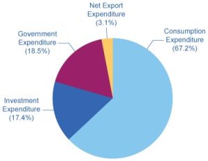
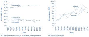
Who buys all of this production? We can divide this demand into four main parts: consumer spending (consumption), business spending (investment), government spending on goods and services, and spending on net exports. (See the following Clear It Up feature to understand what we mean by investment.) Table 19.1 shows how these four components added up to the GDP in 2020, Figure 19.4 (a) shows the levels of consumption, investment, and government purchases over time, expressed as a percentage of GDP, while Figure 19.4 (b) shows the levels of exports and imports as a percentage of GDP over time. A few patterns about each of these components are worth noticing. Table 19.1 shows the components of GDP from the demand side.

Table 19.1 Components of U.S. GDP in 2022: From the Demand Side (Source: http://bea.gov/iTable/index_nipa.cfm, Table 1.1.5)

	Components of GDP on the Demand Side (in trillions of dollars)	Percentage of Total
Consumption	$14.0	67.2%
Investment	$3.6	17.4%
Government	$3.9	18.5%
Exports	$2.1	10.2%
Imports	–$2.7	–13.3%
Total GDP	$20.9	100%

Consumption expenditure by households is the largest component of GDP, accounting for about two-thirds of the GDP in any year. This tells us that consumers’ spending decisions are a major driver of the economy. However, consumer spending is a gentle elephant: when viewed over time, it does not jump around too much, and has increased modestly from about 60% of GDP in the 1960s and 1970s.

Investment expenditure refers to purchases of physical plant and equipment, primarily by businesses. If Starbucks builds a new store, or Amazon buys robots, they count these expenditures under business investment. Investment demand is far smaller than consumption demand, typically accounting for only about 15–18% of GDP, but it is very important for the economy because this is where jobs are created. However, it fluctuates more noticeably than consumption. Business investment is volatile. New technology or a new product can spur business investment, but then confidence can drop and business investment can pull back sharply.

If you have noticed any of the infrastructure projects (new bridges, highways, airports) launched during the 2009 recession, or if you received a stimulus check during the pandemic-induced recession of 2020–2021, you have seen how important government spending can be for the economy. Government expenditure in the United States is close to 20% of GDP, and includes spending by all three levels of government: federal, state, and local. The only part of government spending counted in demand is government purchases of goods or services produced in the economy. Examples include the government buying a new fighter jet for the Air Force (federal government spending), building a new highway (state government spending), or a new school (local government spending). A significant portion of government budgets consists of transfer payments, like unemployment benefits, veteran’s benefits, and Social Security payments to retirees. The government excludes these payments from GDP because it does not receive a new good or service in return or exchange. Instead they are transfers of income from taxpayers to others. If you are curious about the awesome undertaking of adding up GDP, read the following Clear It Up feature.

When thinking about the demand for domestically produced goods in a global economy, it is important to count spending on exports—domestically produced goods that a country sells abroad. Similarly, we must also subtract spending on imports—goods that a country produces in other countries that residents of this country purchase. The GDP net export component is equal to the dollar value of exports (X) minus the dollar value of imports (M), (X – M). We call the gap between exports and imports the trade balance. If a country’s exports are larger than its imports, then a country has a trade surplus. In the United States, exports typically exceeded imports in the 1960s and 1970s, as Figure 19.4(b) shows.

Since the early 1980s, imports have typically exceeded exports, and so the United States has experienced a trade deficit in most years. The trade deficit grew quite large in the late 1990s and in the mid-2000s. Figure 19.4 (b) also shows that imports and exports have both risen substantially in recent decades, even after the declines during the Great Recession between 2008 and 2009. As we noted before, if exports and imports are equal, foreign trade has no effect on total GDP. However, even if exports and imports are balanced overall, foreign trade might still have powerful effects on particular industries and workers by causing nations to shift workers and physical capital investment toward one industry rather than another.

Based on these four components of demand, we can measure GDP as:

 

$$\begin{array}{rcl}\text{GDP}& \text{=}& \text{Consumption + Investment + Government + Trade balance}\\ \text{GDP}& \text{=}& \text{C + I + G + (X – M)}\end{array}$$ Understanding how to measure GDP is important for analyzing connections in the macro economy and for thinking about macroeconomic policy tools.

GDP Measured by What is Produced

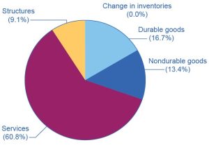
Everything that we purchase somebody must first produce. Table 19.2 breaks down what a country produces into five categories: durable goods, nondurable goods, services, structures, and the change in inventories. Before going into detail about these categories, notice that total GDP measured according to what is produced is exactly the same as the GDP measured by looking at the five components of demand. Figure 19.5 provides a visual representation of this information.

Table 19.2 Components of U.S. GDP on the Production Side, 2020 (Source: http://bea.gov/iTable/index_nipa.cfm, Table 1.2.5)

	Components of GDP on the Supply Side (in trillions of dollars)	Percentage of Total
Goods
Durable goods	$3.5	16.7%
Nondurable goods	$2.8	13.4%
Services	$12.7	60.8%
Structures	$1.9	9.1%
Change in inventories	$0.0	0.0%
Total GDP	$20.9	100%

Since every market transaction must have both a buyer and a seller, GDP must be the same whether measured by what is demanded or by what is produced. Figure 19.6 shows these components of what is produced, expressed as a percentage of GDP, since 1950.

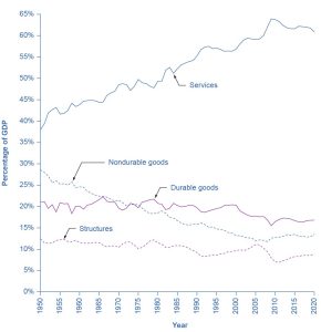
In thinking about what is produced in the economy, many non-economists immediately focus on solid, long-lasting goods, like cars and computers. By far the largest part of GDP, however, is services. Moreover, services have been a growing share of GDP over time. A detailed breakdown of the leading service industries would include healthcare, education, and legal and financial services. It has been decades since most of the U.S. economy involved making solid objects. Instead, the most common jobs in a modern economy involve a worker looking at pieces of paper or a computer screen; meeting with co-workers, customers, or suppliers; or making phone calls.

Even within the overall category of goods, long-lasting durable goods like cars and refrigerators are about the same share of the economy as short-lived nondurable goods like food and clothing. The category of structures includes everything from homes, to office buildings, shopping malls, and factories. Inventories is a small category that refers to the goods that one business has produced but has not yet sold to consumers, and are still sitting in warehouses and on shelves. The amount of inventories sitting on shelves tends to decline if business is better than expected, or to rise if business is worse than expected.

Another Way to Measure GDP: The National Income Approach

GDP is a measure of what is produced in a nation. The primary way GDP is estimated is with the Expenditure Approach we discussed above, but there is another way. Everything a firm produces, when sold, becomes revenues to the firm. Businesses use revenues to pay their bills: Wages and salaries for labor, interest and dividends for capital, rent for land, profit to the entrepreneur, etc. So adding up all the income produced in a year provides a second way of measuring GDP. This is why the terms GDP and national income are sometimes used interchangeably. The total value of a nation’s output is equal to the total value of a nation’s income.

The Problem of Double Counting

We define GDP as the current value of all final goods and services produced in a nation in a year. What are final goods? They are goods at the furthest stage of production at the end of a year. Statisticians who calculate GDP must avoid the mistake of double counting, in which they count output more than once as it travels through the production stages. For example, imagine what would happen if government statisticians first counted the value of tires that a tire manufacturer produces, and then counted the value of a new truck that an automaker sold that contains those tires. In this example, the statisticians would have counted the value of the tires twice-because the truck’s price includes the value of the tires.

To avoid this problem, which would overstate the size of the economy considerably, government statisticians count just the value of final goods and services in the chain of production that are sold for consumption, investment, government, and trade purposes. Statisticians exclude intermediate goods, which are goods that go into producing other goods, from GDP calculations. From the example above, they will only count the Ford truck’s value. The value of what businesses provide to other businesses is captured in the final products at the end of the production chain.

The concept of GDP is fairly straightforward: it is just the dollar value of all final goods and services produced in the economy in a year. In our decentralized, market-oriented economy, actually calculating the more than $21 trillion-dollar U.S. GDP—along with how it is changing every few months—is a full-time job for a brigade of government statisticians.

Table 19.3 Counting GDP

What is Counted in GDP	What is not included in GDP
Consumption	Intermediate goods
Business investment	Transfer payments and non-market activities
Government spending on goods and services	Used goods
Net exports	Illegal goods

Notice the items that are not counted into GDP, as Table 19.3 outlines. The sales of used goods are not included because they were produced in a previous year and are part of that year’s GDP. The entire underground economy of services paid “under the table” and illegal sales should be counted, but is not, because it is impossible to track these sales. In Friedrich Schneider’s recent study of shadow economies, he estimated the underground economy in the United States to be 6.6% of GDP, or close to $2 trillion dollars in 2013 alone. Transfer payments, such as payment by the government to individuals, are not included, because they do not represent production. Also, production of some goods—such as home production as when you make your breakfast—is not counted because these goods are not sold in the marketplace.

Other Ways to Measure the Economy

Besides GDP, there are several different but closely related ways of measuring the size of the economy. We mentioned above that we can think of GDP as total production and as total purchases. We can also think of it as total income since anything one produces and sells yields income.

One of the closest cousins of GDP is the gross national product (GNP). GDP includes only what country produces within its borders. GNP adds what domestic businesses and labor abroad produces, and subtracts any payments that foreign labor and businesses located in the United States send home to other countries. In other words, GNP is based more on what a country’s citizens and firms produce, wherever they are located, and GDP is based on what happens within a certain county’s geographic boundaries. For the United States, the gap between GDP and GNP is relatively small; in recent years, only about 0.2%. For small nations, which may have a substantial share of their population working abroad and sending money back home, the difference can be substantial.

We calculate net national product (NNP) by taking GNP and then subtracting the value of how much physical capital is worn out, or reduced in value because of aging, over the course of a year. The process by which capital ages and loses value is called depreciation. We can further subdivide NNP into national income, which includes all income to businesses and individuals, and personal income, which includes only income to people.

The gross national income (GNI) includes the value of all goods and services produced by people from a country—whether in the country or not. Unlike the other methods, GNI essentially measures the wealth of a nation because it focuses on income, not output. As you will see in the discussion regarding global economic diversity, the World Bank now uses GNI to classify nations according to economic status.

For practical purposes, it is not vital to memorize these definitions. However, it is important to be aware that these differences exist and to know what statistic you are examining, so that you do not accidentally compare, say, GDP in one year or for one country with GNP or NNP in another year or another country. To get an idea of how these calculations work, follow the steps in the following Work It Out feature.

19.2 Adjusting Nominal Values to Real Values

When examining economic statistics, there is a crucial distinction worth emphasizing. The distinction is between nominal and real measurements, which refer to whether or not inflation has distorted a given statistic. Looking at economic statistics without considering inflation is like looking through a pair of binoculars and trying to guess how close something is: unless you know how strong the lenses are, you cannot guess the distance very accurately. Similarly, if you do not know the inflation rate, it is difficult to figure out if a rise in GDP is due mainly to a rise in the overall level of prices or to a rise in quantities of goods produced. The nominal value of any economic statistic means that we measure the statistic in terms of actual prices that exist at the time. The real value refers to the same statistic after it has been adjusted for inflation. Generally, it is the real value that is more important.

Converting Nominal to Real GDP

Table 19.5 shows U.S. GDP at five-year intervals since 1960 in nominal dollars; that is, GDP measured using the actual market prices prevailing in each stated year. Figure 19.7 also reflects this data in a graph.

Table 19.5 U.S. Nominal GDP and the GDP Deflator (Source: https://apps.bea.gov/itable/index.cfm, Table 1.1.5 and Table 1.1.9)

Year	Nominal GDP (billions of dollars)	GDP Deflator (2012 = 100)
1960	542.4	16.6
1965	742.3	17.8
1970	1,073.3	21.7
1975	1,684.9	29.8
1980	2,857.3	42.2
1985	4,339.0	54.5
1990	5,963.1	63.6
1995	7,639.7	71.8
2000	10,251.0	78.0
2005	13,039.2	87.5
2010	15,049.0	96.2
2015	18,206.0	104.7
2020	20,893.7	113.6

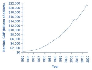
If an unwary analyst compared nominal GDP in 1960 to nominal GDP in 2010, it might appear that national output had risen by a factor of more than 38 over this time (that is, GDP of $20.9 trillion in 2020 divided by GDP of $543 billion in 1960 = 38). This conclusion would be highly misleading. Recall that we define nominal GDP as the quantity of every final good or service produced multiplied by the price at which it was sold, summed up for all goods and services. In order to see how much production has actually increased, we need to extract the effects of higher prices on nominal GDP. We can easily accomplish this using the GDP deflator.

The GDP deflator is a price index measuring the average prices of all final goods and services included in the economy. We explore price indices in detail and how we compute them in Inflation, but this definition will do in the context of this chapter. Table 19.5 provides the GDP deflator data and Figure 19.8 shows it graphically.

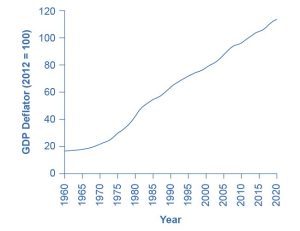
Figure 19.8 shows that the price level has risen dramatically since 1960. The price level in 2020 was seven times higher than in 1960 (the deflator for 2020 was 113 versus a level of 17 in 1960). Clearly, much of the growth in nominal GDP was due to inflation, not an actual change in the quantity of goods and services produced, in other words, not in real GDP. Recall that nominal GDP can rise for two reasons: an increase in output, and/or an increase in prices. What is needed is to extract the increase in prices from nominal GDP so as to measure only changes in output. After all, the dollars used to measure nominal GDP in 1960 are worth more than the inflated dollars of 2020—and the price index tells exactly how much more. This adjustment is easy to do if you understand that nominal measurements are in value terms, where

$$\begin{array}{rcll}\text{Value}& \text{=}& \text{Price × Quantity}& \\ & & \text{or}& \\ \text{Nominal GDP}& \text{=}& \text{GDP Deflator × Real GDP}& \end{array}$$ 

Let’s look at an example at the micro level. Suppose the t-shirt company, Coolshirts, sells 10 t-shirts at a price of $9 each.

$$\begin{array}{rcl}\text{Coolshirt’s nominal revenue from sales}& \text{=}& \text{Price × Quantity}\\ & \text{=}& \text{\$9 × 10}\\ & \text{=}& \text{\$90}\end{array}$$ Then,

$$\begin{array}{lcl}\text{Coolshirt’s real income}& \text{=}& \frac{\text{Nominal revenue}}{\text{Price}}\\ & \text{=}& \frac{\text{\$90}}{\text{\$9}}\\ & \text{=}& \text{10}\end{array}$$ In other words, when we compute “real” measurements we are trying to obtain actual quantities, in this case, 10 t-shirts.

With GDP, it is just a tiny bit more complicated. We start with the same formula as above:

 

$$\begin{array}{rcl}\text{Real GDP}& \text{=}& \frac{\text{Nominal GDP}}{\text{Price Index}}\end{array}$$ For reasons that we will explain in more detail below, mathematically, a price index is a two-digit decimal number like 1.00 or 0.85 or 1.25. Because some people have trouble working with decimals, when the price index is published, it has traditionally been multiplied by 100 to get integer numbers like 100, 85, or 125. What this means is that when we “deflate” nominal figures to get real figures (by dividing the nominal by the price index). We also need to remember to divide the published price index by 100 to make the math work. Thus, the formula becomes:

 

$$\begin{array}{rcl}\text{Real GDP}& \text{=}& \frac{\text{Nominal GDP}}{\text{Price Index / 100}}\end{array}$$ Now read the following Work It Out feature for more practice calculating real GDP.

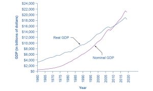
Figure 19.9 shows the U.S. nominal and real GDP since 1960. Because 2005 is the base year, the nominal and real values are exactly the same in that year. However, over time, the rise in nominal GDP looks much larger than the rise in real GDP (that is, the nominal GDP line rises more steeply than the real GDP line), because the presence of inflation, especially in the 1970s exaggerates the rise in nominal GDP.

Let’s return to the question that we posed originally: How much did GDP increase in real terms? What was the real GDP growth rate from 1960 to 2020? To find the real growth rate, we apply the formula for percentage change:

 

$$\begin{array}{rcl}\frac{\text{2020 real GDP – 1960 real GDP}}{\text{1960 real GDP}}\text{× 100}& \text{=}& \text{\% change}\\ \frac{\text{18,392.3 – 3,267.5}}{\text{3,267.5}}\text{× 100}& \text{=}& \text{463\%}\end{array}$$ In other words, the U.S. economy has increased real production of goods and services by nearly a factor of five since 1960. Of course, that understates the material improvement since it fails to capture improvements in the quality of products and the invention of new products.

There is a quicker way to answer this question approximately, using another math trick. Because:

 

$$\begin{array}{rcl}\text{Nominal}& \text{=}& \text{Price × Quantity}\\ \text{\% change in Nominal}& \text{=}& \text{\% change in Price + \% change in Quantity}\\ & \text{OR}& \\ \text{\% change in Quantity}& \text{=}& \text{\% change in Nominal – \% change in Price}\end{array}$$ Therefore, real GDP growth rate (% change in quantity) equals the growth rate in nominal GDP (% change in value) minus the inflation rate (% change in price).

Note that using this equation provides an approximation for small changes in the levels. For more accurate measures, one should use the first formula.

19.3 Tracking Real GDP over Time

When news reports indicate that “the economy grew 1.2% in the first quarter,” the reports are referring to the percentage change in real GDP. By convention, governments report GDP growth at an annualized rate: Whatever the calculated growth in real GDP was for the quarter, we multiply it by four when it is reported as if the economy were growing at that rate for a full year.

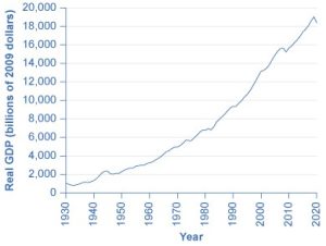
Figure 19.10 shows the pattern of U.S. real GDP since 1930. Short term declines have regularly interrupted the generally upward long-term path of GDP. We call a significant decline in real GDP a recession. We call an especially lengthy and deep recession a depression. The severe drop in GDP that occurred during the 1930s Great Depression is clearly visible in the figure, as is the 2008–2009 Great Recession and the recession induced by COVID-19 in 2020.

Real GDP is important because it is highly correlated with other measures of economic activity, like employment and unemployment. When real GDP rises, so does employment.

The most significant human problem associated with recessions (and their larger, uglier cousins, depressions) is that a slowdown in production means that firms need to lay off or fire some of their workers. Losing a job imposes painful financial and personal costs on workers, and often on their extended families as well. In addition, even those who keep their jobs are likely to find that wage raises are scanty at best—or their employers may ask them to take pay cuts.

Table 19.7 lists the pattern of recessions and expansions in the U.S. economy since 1900. We call the highest point of the economy, before the recession begins, the peak. Conversely, the lowest point of a recession, before a recovery begins, is the trough. Thus, a recession lasts from peak to trough, and an economic upswing runs from trough to peak. We call the economy’s movement from peak to trough and trough to peak the business cycle. It is intriguing to notice that the three longest trough-to-peak expansions of the twentieth century have happened since 1960. The most recent recession was caused by the COVID-19 pandemic. It started in February 2020 and ended formally in May 2020. This was the most severe recession since the 1930s Great Depression, but also the shortest. The previous recession, called the Great Recession, was also very severe and lasted about 18 months. The expansion starting in June 2009, the trough from the Great Recession, was the longest on record—ending 128 months with the pandemic-induced recession.

Table 19.7 U.S. Business Cycles since 1900 (Source: http://www.nber.org/cycles/main.html)

Trough	Peak	Months of Contraction	Months of Expansion
December 1900	September 1902	18	21
August 1904	May 1907	23	33
June 1908	January 1910	13	19
January 1912	January 1913	24	12
December 1914	August 1918	23	44
March 1919	January 1920	7	10
July 1921	May 1923	18	22
July 1924	October 1926	14	27
November 1927	August 1929	23	21
March 1933	May 1937	43	50
June 1938	February 1945	13	80
October 1945	November 1948	8	37
October 1949	July 1953	11	45
May 1954	August 1957	10	39
April 1958	April 1960	8	24
February 1961	December 1969	10	106
November 1970	November 1973	11	36
March 1975	January 1980	16	58
July 1980	July 1981	6	12
November 1982	July 1990	16	92
March 1991	March 2001	8	120
November 2001	December 2007	8	73
January 2009	February 2020	2	128
April 2020	TBD	TBD	TBD

A private think tank, the National Bureau of Economic Research (NBER), tracks business cycles for the U.S. economy. However, the effects of a severe recession often linger after the official ending date assigned by the NBER.

19.4 Comparing GDP among Countries

It is common to use GDP as a measure of economic welfare or standard of living in a nation. When comparing the GDP of different nations for this purpose, two issues immediately arise. First, we measure a country’s GDP in its own currency: the United States uses the U.S. dollar; Canada, the Canadian dollar; most countries of Western Europe, the euro; Japan, the yen; Mexico, the peso; and so on. Thus, comparing GDP between two countries requires converting to a common currency. A second issue is that countries have very different numbers of people. For instance, the United States has a much larger economy than Mexico or Canada, but it also has almost three times as many people as Mexico and nine times as many people as Canada. Thus, if we are trying to compare standards of living across countries, we need to divide GDP by population.

Converting Currencies with Exchange Rates

To compare the GDP of countries with different currencies, it is necessary to convert to a “common denominator” using an exchange rate, which is the value of one currency in terms of another currency. We express exchange rates either as the units of country A’s currency that need to be traded for a single unit of country B’s currency (for example, Japanese yen per British pound), or as the inverse (for example, British pounds per Japanese yen). We can use two types of exchange rates for this purpose, market exchange rates and purchasing power parity (PPP) equivalent exchange rates. Market exchange rates vary on a day-to-day basis depending on supply and demand in foreign exchange markets. PPP-equivalent exchange rates provide a longer run measure of the exchange rate. For this reason, economists typically use PPP-equivalent exchange rates for GDP cross country comparisons. We will discuss exchange rates in more detail in Exchange Rates and International Capital Flows. The following Work It Out feature explains how to convert GDP to a common currency.

GDP Per Capita

The U.S. economy has the largest GDP in the world, by a considerable amount. The United States is also a populous country; in fact, it is the third largest country by population in the world, although well behind China and India. Is the U.S. economy larger than other countries just because the United States has more people than most other countries, or because the U.S. economy is actually larger on a per-person basis? We can answer this question by calculating a country’s GDP per capita; that is, the GDP divided by the population.

$$\begin{array}{rcl}\text{GDP per capita}& \text{ = }& \text{GDP/population}\end{array}$$

The second column of Table 19.9 lists the GDP of the same selection of countries that appeared in the previous Tracking Real GDP over Time and Table 19.8, showing their GDP as converted into U.S. dollars (which is the same as the last column of the previous table). The third column gives the population for each country. The fourth column lists the GDP per capita. We obtain GDP per capita in two steps: First, by multiplying column two (GDP, in billions of dollars) by 1000 so it has the same units as column three (Population, in millions). Then divide the result (GDP in millions of dollars) by column three (Population, in millions).

Table 19.9 GDP Per Capita, 2020 (Source: https://data.worldbank.org/indicator/NY.GDP.MKTP.CD)

Country	GDP (in billions of U.S. dollars)	Population (in millions)	Per Capita GDP (in U.S. dollars)
Brazil	3,153.60	212.56	14,836.27
Canada	1,827.71	38.00	48,097.62
China	24,273.36	1,402.11	17,312.02
Egypt	1,290.21	102.33	12,608.30
Germany	4,516.94	83.24	54,263.99
India	8,907.03	1,380.00	6,454.37
Japan	5,166.00	125.84	41,052.13
Mexico	2,428.20	128.93	18,833.48
South Korea	2,233.00	51.78	43,124.78
United Kingdom	3,019.60	67.22	44,913.08
United States	20,936.60	329.48	63,544.37

Notice that the rankings by GDP in billions of U.S. dollars, and by GDP per capita, are different than the ranking of GDP by each country’s currency. Measured by its own currency, the rupee, India has a somewhat larger GDP than Germany. On a per capita basis in U.S. dollars, Germany has more than 9 times India’s per capita GDP on PPP terms.

The world’s high-income nations—including the United States, Canada, the Western European countries, and Japan—typically have GDP per capita in the range of $20,000 to $50,000. Middle-income countries, which include much of Latin America, Eastern Europe, and some countries in East Asia, have GDP per capita in the range of $6,000 to $12,000. The world’s low-income countries, many of them located in Africa and Asia, often have GDP per capita of less than $2,000 per year.

19.5 How Well GDP Measures the Well-Being of Society

The level of GDP per capita clearly captures some of what we mean by the phrase “standard of living.” Most of the migration in the world, for example, involves people who are moving from countries with relatively low GDP per capita to countries with relatively high GDP per capita.

“Standard of living” is a broader term than GDP. While GDP focuses on production that is bought and sold in markets, standard of living includes all elements that affect people’s well-being, whether they are bought and sold in the market or not. To illuminate the difference between GDP and standard of living, it is useful to spell out some things that GDP does not cover that are clearly relevant to standard of living.

Limitations of GDP as a Measure of the Standard of Living

GDP measures economic activity, not all activity. As a result, economists like Kate Raworth see it as a somewhat outdated and limited indication of well-being and prosperity. While GDP measures output of work done at home, as well as spending on travel, it doesn’t capture unpaid work or leisure time. So, two countries may have equal GDP, but one nation’s workers may have an average workday of eight hours, while the other has an average workday of twelve hours. In that case, is their equal GDP truly measuring the prosperity of those nations? The GDP per capita of the U.S. economy is larger than the GDP per capita of Germany, as Table 19.9 showed, but does that prove that the standard of living in the United States is higher? Not necessarily, since it is also true that the average U.S. worker works several hundred hours more per year more than the average German worker. Calculating GDP does not account for the German worker’s extra vacation weeks.

While GDP includes what a country spends on environmental protection, healthcare, and education, it does not include actual levels of environmental cleanliness, health, and learning. GDP includes the cost of buying pollution-control equipment, but it does not address whether the air and water are actually cleaner or dirtier. GDP includes spending on medical care, but does not address whether life expectancy or infant mortality have risen or fallen. Similarly, it counts spending on education, but does not address directly how much of the population can read, write, or do basic mathematics.

GDP includes production that is exchanged in the market, but it does not cover production that is not exchanged in the market. For example, hiring someone to mow your lawn or clean your house is part of GDP, but doing these tasks yourself is not part of GDP. One remarkable change in the U.S. economy in recent decades is the growth in women’s participation in the labor force. As of 1970, only about 42% of women participated in the paid labor force. By the second decade of the 2000s, nearly 60% of women participated in the paid labor force according to the Bureau of Labor Statistics. As women are now in the labor force, many of the services they used to produce in the non-market economy like food preparation and child care have shifted to some extent into the market economy, which makes the GDP appear larger even if people actually are not consuming more services. However, as Raworth points out and was explored in the chapter on the labor market, even women who are fully employed expend significant effort (generally more than men) in raising children and maintaining a home. Raworth advocates that economic measures include monetized and un-monetized goods and services, so that the status and contributors to each economy are more accurate.

GDP has nothing to say about the level of inequality in society. GDP per capita is only an average. When GDP per capita rises by 5%, it could mean that GDP for everyone in the society has risen by 5%, or that GDP of some groups has risen by more while that of others has risen by less—or even declined. GDP also has nothing in particular to say about the amount of variety available. If a family buys 100 loaves of bread in a year, GDP does not care whether they are all white bread, or whether the family can choose from wheat, rye, pumpernickel, and many others—it just looks at the total amount the family spends on bread.

Likewise, GDP has nothing much to say about what technology and products are available. The standard of living in, for example, 1950 or 1900 was not affected only by how much money people had—it was also affected by what they could buy. No matter how much money you had in 1950, you could not buy an iPhone or a personal computer.

In certain cases, it is not clear that a rise in GDP is even a good thing. If a city is wrecked by a hurricane, and then experiences a surge of rebuilding construction activity, it would be peculiar to claim that the hurricane was therefore economically beneficial. If people are led by a rising fear of crime, to pay for installing bars and burglar alarms on all their windows, it is hard to believe that this increase in GDP has made them better off. Similarly, some people would argue that sales of certain goods, like pornography or extremely violent movies, do not represent a gain to society’s standard of living.

Does a Rise in GDP Overstate or Understate the Rise in the Standard of Living?

The fact that GDP per capita does not fully capture the broader idea of standard of living has led to a concern that the increases in GDP over time are illusory. It is theoretically possible that while GDP is rising, the standard of living could be falling if human health, environmental cleanliness, and other factors that are not included in GDP are worsening. Fortunately, this fear appears to be overstated.

In some ways, the rise in GDP understates the actual rise in the standard of living. For example, the typical workweek for a U.S. worker has fallen over the last century from about 60 hours per week to less than 40 hours per week. Life expectancy and health have risen dramatically, and so has the average level of education. Since 1970, the air and water in the United States have generally been getting cleaner. Companies have developed new technologies for entertainment, travel, information, and health. A much wider variety of basic products like food and clothing is available today than several decades ago. Because GDP does not capture leisure, health, a cleaner environment, the possibilities that new technology creates, or an increase in variety, the actual rise in the standard of living for Americans in recent decades has exceeded the rise in GDP.

On the other side, crime rates, traffic congestion levels, and income inequality are higher in the United States now than they were in the 1960s. Moreover, a substantial number of services that women primarily provided in the non-market economy are now part of the market economy that GDP counts. By ignoring these factors, GDP would tend to overstate the true rise in the standard of living.

GDP is Rough, but Useful

A high level of GDP should not be the only goal of macroeconomic policy, or government policy more broadly. Even though GDP does not measure the broader standard of living with any precision, it does measure production well and it does indicate when a country is materially better or worse off in terms of jobs and incomes. In most countries, a significantly higher GDP per capita occurs hand in hand with other improvements in everyday life along many dimensions, like education, health, and environmental protection.

No single number can capture all the elements of a term as broad as “standard of living.” Nonetheless, GDP per capita is a reasonable, rough-and-ready measure of the standard of living.