Crit Research Worksheet

What Are Statistics?

Statistics include numerical facts and figures. For instance:

• The largest earthquake measured 9.2 on the Richter scale.
• Men are at least 10 times more likely than women to commit murder.
• One in every eight South Africans is HIV positive.
• By the year 2050, there will be 12 people aged 65 and over for every new baby born.

The study of statistics involves math and relies upon calculations of numbers. But it also relies heavily on how the numbers are chosen and how the statistics are interpreted. For example, consider the following three scenarios and the interpretations based on the presented statistics. You will find that the numbers may be right, but the interpretation may be wrong. Try to identify a major flaw with each interpretation before we describe it.

1. A new advertisement for Ben & Jerry’s ice cream introduced in late May of last year resulted in a 30% increase in ice cream sales for the following three months. Thus, the advertisement was effective.
   Major flaw: Ice cream consumption generally increases in the months of June, July, and August, regardless of advertisements. This effect is called a history effect and leads people to interpret outcomes as the result of one variable when another variable (in this case, one having to do with the passage of time) is actually responsible.
2. The more churches in a city, the more crime there is. Thus, churches lead to crime.
   Major flaw: Both increased churches and increased crime rates can be explained by larger populations. In bigger cities, there are both more churches and more crime. This problem, which we will discuss in more detail in the chapter on sampling, refers to the third-variable problem. Namely, a third variable can cause both situations; however, people erroneously believe that there is a causal relationship between the two primary variables rather than recognizing that a third variable can cause both.
3. Seventy-five percent more interracial marriages are occurring this year than 25 years ago. Thus, our society accepts interracial marriages.
   Major flaw: We don’t have the information we need. What is the rate at which marriages are occurring? Suppose only 1% of marriages 25 years ago were interracial, and so now 1.75% of marriages are interracial (1.75 is 75% higher than 1). But this latter number is hardly evidence suggesting the acceptability of interracial marriages. In addition, the statistic provided does not rule out the possibility that the number of interracial marriages has seen dramatic fluctuations over the years, and this year is not the highest. Again, there is simply not enough information to understand fully the impact of the statistics.

As a whole, these examples show that statistics are not only facts and figures; they are something more than that. In the broadest sense, “statistics” refers to a range of techniques and procedures for analyzing, interpreting, displaying, and making decisions based on data.

Statistics is the language of science and data. The ability to understand and communicate using statistics enables researchers from different labs, different languages, and different fields to articulate to one another exactly what they have found in their work. It is an objective, precise, and powerful tool in science and in everyday life.

What a Statistics Course Is Not

Many psychology students dread the idea of taking a statistics course, and more than a few have changed majors upon learning that it is a requirement. That is because many students view statistics as a math class, which is actually not true. While many of you will not believe this or agree with it, statistics isn’t math.

Although math is a central component of it, statistics is a broader way of organizing, interpreting, and communicating information in an objective manner. Indeed, great care has been taken to eliminate as much math from this course as possible (students who do not believe this are welcome to ask the professor what matrix algebra is). Statistics is a way of viewing reality as it exists around us in a way that we otherwise could not.

Why Do We Study Statistics?

Virtually every student of the behavioral sciences takes some form of statistics class. This is because statistics is how we communicate in science. It serves as the link between a research idea and usable conclusions. Without statistics, we would be unable to interpret the massive amounts of information contained in data. Even small datasets contain hundreds—if not thousands—of numbers, each representing a specific observation we made. Without a way to organize these numbers into a more interpretable form, we would be lost, having wasted the time and money of our participants, ourselves, and the communities we serve.

Beyond its use in science, however, there is a more personal reason to study statistics. Like most people, you probably feel that it is important to “take control of your life.” But what does this mean? Partly, it means being able to properly evaluate the data and claims that bombard you every day. If you cannot distinguish good from faulty reasoning, then you are vulnerable to manipulation and to decisions that are not in your best interest. Statistics provides tools that you need in order to react intelligently to information you hear or read. In this sense, statistics is one of the most important things that you can study.

To be more specific, here are some claims that we have heard on several occasions. (We are not saying that each one of these claims is true!)

• Four out of five dentists recommend Dentine.
• Almost 85% of lung cancers in men and 45% in women are tobacco-related.
• Condoms are effective 94% of the time.
• People tend to be more persuasive when they look others directly in the eye and speak loudly and quickly.
• Women make 75 cents to every dollar a man makes when they work the same job.
• A surprising new study shows that eating egg whites can increase one’s life span.
• People predict that it is very unlikely there will ever be another baseball player with a batting average over 400.
• There is an 80% chance that in a room full of 30 people at least two people will share the same birthday.
• 79.48% of all statistics are made up on the spot.

All of these claims are statistical in character. We suspect that some of them sound familiar; if not, we bet that you have heard other claims like them. Notice how diverse the examples are. They come from psychology, health, law, sports, business, etc. Indeed, data and data interpretation show up in discourse from virtually every facet of contemporary life.

Statistics are often presented in an effort to add credibility to an argument or advice. You can see this by paying attention to television advertisements. Many of the numbers thrown about in this way do not represent careful statistical analysis. They can be misleading and push you into decisions that you might find cause to regret. For these reasons, learning about statistics is a long step toward taking control of your life. (It is not, of course, the only step needed to do so.) The purpose of this course, beyond preparing you for a career in psychology, is to help you learn statistical essentials. It will make you into an intelligent consumer of statistical claims.

You can take the first step right away. To be an intelligent consumer of statistics, your first reflex must be to question the statistics you encounter. The British Prime Minister Benjamin Disraeli is quoted by Mark Twain as having said, “There are three kinds of lies—lies, damned lies, and statistics.” This quote reminds us why it is so important to understand statistics. So let us invite you to reform your statistical habits from now on. No longer will you blindly accept numbers or findings. Instead, you will begin to think about the numbers, their sources, and most importantly, the procedures used to generate them.

The above section puts an emphasis on defending ourselves against fraudulent claims wrapped up as statistics, but let us look at a more positive note. Just as important as detecting the deceptive use of statistics is the appreciation of the proper use of statistics. You must also learn to recognize statistical evidence that supports a stated conclusion. Statistics are all around you, sometimes used well, sometimes not. We must learn how to distinguish the two cases. In doing so, statistics will likely be the course you use most in your day-to-day life, even if you do not ever run a formal analysis again.

Types of Statistical Analyses

Now that we understand the nature of our data, let’s turn to the types of statistics we can use to interpret them. There are two types of statistics: descriptive and inferential.

Descriptive Statistics

Descriptive statistics are numbers that are used to summarize and describe data. The word “data” refers to the information that has been collected from an experiment, a survey, a historical record, etc. (By the way, data is plural. One piece of information is called a datum.) If we are analyzing birth certificates, for example, a descriptive statistic might be the percentage of certificates issued in New York State or the average age of the mother. Any other number we choose to compute also counts as a descriptive statistic for the data from which the statistic is computed. Several descriptive statistics are often used at one time to give a full picture of the data.

Descriptive statistics are just descriptive. They do not involve generalizing beyond the data at hand. Generalizing from our data to another set of cases is the business of inferential statistics, which you’ll be studying in another section. Here we focus on (mere) descriptive statistics.

Some descriptive statistics are shown in Table 24.1. The table shows the average salaries for various occupations in the United States in 1999. Descriptive statistics like these offer insight into American society. It is interesting to note, for example, that we pay the people who educate our children and who protect our citizens a great deal less than we pay people who take care of our feet or our teeth.

For more descriptive statistics, consider Table 24.2. It shows the number of unmarried men per 100 unmarried women in U.S. metro areas in 1990. From this table we see that men outnumber women most in Jacksonville, North Carolina, and women outnumber men most in Sarasota, Florida. You can see that descriptive statistics can be useful if we are looking for an opposite-sex partner! (These data come from the Information Please Almanac.)

These descriptive statistics may make us ponder why the numbers are so disparate in these cities. One potential explanation, for instance, as to why there are more women in Florida than men may involve the fact that elderly individuals tend to move down to the Sarasota region and that women tend to outlive men. Thus, more women might live in Sarasota than men. However, in the absence of proper data, this is only speculation.

You probably know that descriptive statistics are central to the world of sports. Every sporting event produces numerous statistics, such as the shooting percentage of players on a basketball team. For the Olympic marathon (a foot race of 26.2 miles), we possess data that cover more than a century of competition. (The first modern Olympics took place in 1896.) Table 24.3 and Table 24.4 show the winning times for women and men, respectively. (Women have only been allowed to compete since 1984.)

Table 24.3. Women’s winning Olympic marathon times, 1984–2004.

Year	Winner	Country	Time
1984	Joan Benoit	United States	2:24:52
1988	Rosa Mota	Portugal	2:25:40
1992	Valentina Yegorova	Unified Team	2:32:41
1996	Fatuma Roba	Ethiopia	2:26:05
2000	Naoko Takahashi	Japan	2:23:14
2004	Mizuki Noguchi	Japan	2:26:20

Table 24.4. Men’s winning Olympic marathon times, 1896–2004.

Year	Winner	Country	Time
1896	Spyridon Louis	Greece	2:58:50
1900	Michel Théato	France	2:59:45
1904	Thomas Hicks	United States	3:28:53
1906	Billy Sherring	Canada	2:51:23
1908	Johnny Hayes	United States	2:55:18
1912	Kenneth McArthur	South Africa	2:36:54
1920	Hannes Kolehmainen	Finland	2:32:35
1924	Albin Stenroos	Finland	2:41:22
1928	Boughera El Ouafi	France	2:32:57
1932	Juan Carlos Zabala	Argentina	2:31:36
1936	Sohn Kee-chung	Japan	2:29:19
1948	Delfo Cabrera	Argentina	2:34:51
1952	Emil Zátopek	Czechoslovakia	2:23:03
1956	Alain Mimoun	France	2:25:00
1960	Abebe Bikila	Ethiopia	2:15:16
1964	Abebe Bikila	Ethiopia	2:12:11
1968	Mamo Wolde	Ethiopia	2:20:26
1972	Frank Shorter	United States	2:12:19
1976	Waldemar Cierpinski	East Germany	2:09:55
1980	Waldemar Cierpinski	East Germany	2:11:03
1984	Carlos Lopes	Portugal	2:09:21
1988	Gelindo Bordin	Italy	2:10:32
1992	Hwang Young-cho	South Korea	2:13:23
1996	Josia Thugwane	South Africa	2:12:36
2000	Gezahegne Abera	Ethiopia	2:10.10
2004	Stefano Baldini	Italy	2:10:55

There are many descriptive statistics that we can compute from the data in these tables. To gain insight into the improvement in speed over the years, let us divide the men’s times into two pieces, namely, the first 13 races (up to 1952) and the second 13 (starting from 1956). The mean winning time for the first 13 races is 2 hours, 44 minutes, and 22 seconds (written 2:44:22). The mean winning time for the second 13 races is 2:13:18. This is quite a difference (over half an hour). Does this prove that the fastest men are running faster? Or is the difference just due to chance, no more than what often emerges from chance differences in performance from year to year? We can’t answer this question with descriptive statistics alone. All we can affirm is that the two means are “suggestive.”

Examining Table 24.3 and Table 24.4 leads to many other questions. We note that Takahashi (the lead female runner in 2000) would have beaten the male runner in 1956 and all male runners in the first 12 marathons. This fact leads us to ask whether the gender gap will close or remain constant. When we look at the times within each gender, we also wonder how far they will decrease (if at all) in the next century of the Olympics. Might we one day witness a sub-2-hour marathon? The study of statistics can help you make reasonable guesses about the answers to these questions.

To summarize, there are a variety of ways that statisticians use to describe a data set:

• Exploratory data analysis uses graphs and numerical summaries to describe the variables and their relationship to each other. You will learn how to organize a data set by grouping the data into intervals called classes and forming a frequency distribution.
• Center of the Data uses measures of central tendency to locate the middle or center of a distribution where most of the data tends to be concentrated. The three best-known measures of central tendency used by statisticians are discussed later in this section of the text: the mean, median, and mode.
• Spread of the Data uses measures of variability to describe how far apart data points lie from each other and from the center of the distribution. The section on variability discusses the four most common measures of variability: range, interquartile range, variance, and standard deviation.
• Shape of the Data can be either symmetrical (the normal distribution) or skewed (positive or negative). The section on probability and the normal distribution reveals how the shape of the distribution can easily be discernible through graphs.
• Fractiles or Quantiles of the Data uses measures of position that partition, or divide, an ordered data set into equal parts: first, second, and third quartile; percentiles; and the standard score (z-score). A fractile is a point where a specified proportion of the data lies below that point. Section 2.5 discusses how fractiles are used to specify the position of a data point within a data set.

It is also important to differentiate what we use to describe populations vs. what we use to describe samples. A population is described by a parameter; the parameter is the true value of the descriptive in the population, but one that we can never know for sure. For example, the Bureau of Labor Statistics reports that the average hourly wage of chefs is $23.87. However, even if this number were computed using information from every single chef in the United States (making it a parameter), it would quickly become slightly off as one chef retires and a new chef enters the job market. Additionally, as noted above, there is virtually no way to collect data from every single person in a population. In order to understand a variable, we estimate the population parameter using a sample statistic. Here, the term statistic refers to the specific number we compute from the data (e.g., the average), not the field of statistics. A sample statistic is an estimate of the true population parameter, and if our sample is representative of the population, then the statistic is considered to be a good estimator of the parameter.

Even the best sample will be somewhat off from the full population, earlier referred to as sampling bias, and as a result, there will always be a tiny discrepancy between the parameter and the statistic we use to estimate it. This difference is known as sampling error, and, as we will see throughout the course, understanding sampling error is the key to understanding statistics. Every observation we make about a variable, be it a full research study or observing an individual’s behavior, is incapable of being completely representative of all possibilities for that variable. Knowing where to draw the line between an unusual observation and a true difference is what statistics is all about.

Inferential Statistics

Descriptive statistics are wonderful at telling us what our data look like. However, what we often want to understand is how our data behave. What variables are related to other variables? Under what conditions will the value of a variable change? Are two groups different from each other, and if so, are people within each group different or similar? These are the questions answered by inferential statistics, and inferential statistics are how we generalize from our sample back up to our population. Unit 2 and Unit 3 are all about inferential statistics, the formal analyses and tests we run to make conclusions about our data.

For example, we will learn how to use a t-statistic to determine whether people change over time when enrolled in an intervention. We will also use an F-statistic to determine if we can predict future values of a variable based on current known values of a variable. There are many types of inferential statistics, each allowing us insight into a different behavior of the data we collect. This course will only touch on a small subset (or a sample) of them, but the principles we learn along the way will make it easier to learn new tests, as most inferential statistics follow the same structure and format.

A Note about Statistical Software

Many pieces of technology support statistical analysis and quantitative data analysis done by psychologists. Commonly used technologies include the proprietary Statistical Package for the Social Sciences (SPSS), the free and open-source tool JASP, and the programming language R. Several of the figures used in this text were generated using JASP, but providing an overview or introduction to these technologies is outside the scope of this work. Instruction manuals can be found on the JASP website.

Mathematical Notation

As noted earlier, statistics is not math. It does, however, use math as a tool. Many statistical formulas involve summing numbers. Fortunately, there is a convenient notation for expressing summation. This section covers the basics of this summation notation.

Let’s say we have a variable X that represents the weights (in grams) of 4 grapes:

Table 24.5. Weight of Grapes

Grape	X
Grape 1	4.6
Grape 2	5.1
Grape 3	4.9
Grape 4	4.4

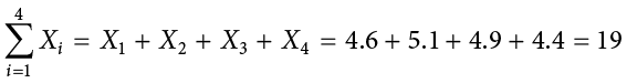
We label the weight of Grape 1 as , of Grape 2 as , etc. The following formula means to sum up the weights of the four grapes:

The Greek letter indicates summation. The “i = 1” at the bottom indicates that the summation is to start with , and the 4 at the top indicates that the summation will end with . The “” indicates that X is the variable to be summed as i goes from 1 to 4. Therefore,

The symbol

indicates that only the first 3 scores are to be summed. The index variable i goes from 1 to 3.

When all the scores of a variable (such as X) are to be summed, it is often convenient to use the following abbreviated notation:

Thus, when no values of i are shown, it means to sum all the values of X.

Many formulas involve squaring numbers before they are summed. This is indicated as

Notice that:

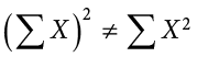
because the expression on the left means to sum up all the values of X and then square the sum (), whereas the expression on the right means to square the numbers and then sum the squares (90.54, as shown).

Some formulas involve the sum of cross products. Below are the data for variables X and Y. The cross products (XY) are shown in the third column. The sum of the cross products is .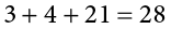

Table 24.6. Values of X and Y and Their Cross Products

X	Y	XY
1	3	3
2	2	4
3	7	21

In summation notation, this is written as: