Introduction to Environmental Protection and Negative Externalities

In 1969, the Cuyahoga River in Ohio was so polluted that it spontaneously burst into flame. Air pollution was so bad at that time that Chattanooga, Tennessee, was a city where, as an article from Sports Illustrated put it:

the death rate from tuberculosis was double that of the rest of Tennessee and triple that of the rest of the United States, a city in which the filth in the air was so bad it melted nylon stockings off women’s legs, in which executives kept supplies of clean white shirts in their offices so they could change when a shirt became too gray to be presentable, in which headlights were turned on at high noon because the sun was eclipsed by the gunk in the sky.

The problem of pollution arises for every economy in the world, whether it is high income or low income, market oriented or command oriented. Every country needs to strike a balance between production and environmental quality. This chapter begins by discussing how firms may fail to take certain social costs, such as pollution, into their planning if they do not need to pay these costs. Traditionally, policies for environmental protection have focused on governmental limits on how much of each pollutant can be emitted. Although this approach has had some success, economists have suggested a range of more flexible, market-oriented policies that reduce pollution at a lower cost. We will consider both approaches, but first, let’s see how economists frame and analyze these issues.

12.1 The Economics of Pollution

Between 1970 and 2020, the U.S. population increased by 63%, and the size of the U.S. economy increased by more than 3.8 times. Since the 1970s, however, the United States, using a variety of antipollution policies, has made genuine progress against a number of pollutants. Table 12.1 lists the change in carbon dioxide emissions by energy users (from residential to industrial) according to the U.S. Energy Information Administration (EIA). The table shows that emissions of certain key air pollutants declined substantially from 2007 to 2012. They dropped 740 million metric tons a year, which is a 12% reduction. This seems to indicate that progress has been made in the United States in reducing overall carbon dioxide emissions, which contribute to the greenhouse effect.

Despite the gradual reduction in emissions from fossil fuels, many important environmental issues remain. Along with the still high levels of air and water pollution, other issues include hazardous waste disposal, destruction of wetlands and other wildlife habitats, and the impact on human health from pollution.

Externalities

Private markets, such as the cell phone industry, offer an efficient way to put buyers and sellers together and determine what goods they produce, how they produce them, and who gets them. The principle that voluntary exchange benefits both buyers and sellers is a fundamental building block of the economic way of thinking. However, what happens when a voluntary exchange affects a third party who is neither the buyer nor the seller?

As an example, consider a concert producer who wants to build an outdoor arena that will host country music concerts a half-mile from your neighborhood. You will be able to hear these outdoor concerts while sitting on your back porch—or perhaps even in your dining room. In this case, the sellers and buyers of concert tickets may both be quite satisfied with their voluntary exchange, but you have no voice in their market transaction. The effect of a market exchange on a third party who is outside or “external” to the exchange is called an externality. Because externalities that occur in market transactions affect other parties beyond those involved, they are sometimes called spillovers.

Externalities can be negative or positive. If you hate country music, then having it waft into your house every night would be a negative externality. If you love country music, then what amounts to a series of free concerts would be a positive externality.

Pollution as a Negative Externality

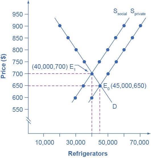
Pollution is a negative externality. Economists illustrate the social costs of production with a demand and supply diagram. The social costs include the private costs of production that a company incurs and the external costs of pollution that are passed on to society. Figure 12.2 shows the demand and supply for manufacturing refrigerators. The demand curve (D) shows the quantity demanded at each price. The supply curve (S_private) shows the quantity of refrigerators that all firms in the industry supply at each price, assuming they are taking only their private costs into account and they are allowed to emit pollution at zero cost. The market equilibrium (E₀), where quantity supplied equals quantity demanded, is at a price of $650 per refrigerator and a quantity of 45,000 refrigerators. Table 12.2 reflects this information in the first three columns.

However, as a by-product of the metals, plastics, chemicals, and energy that refrigerator manufacturers use, some pollution is created. Let’s say that, if these pollutants were emitted into the air and water, they would create costs of $100 per refrigerator produced. These costs might occur because of adverse effects on human health, property values, or wildlife habitat; reduction of recreation possibilities; or other negative impacts. In a market with no antipollution restrictions, firms can dispose of certain wastes for free. Now, imagine that firms that produce refrigerators must factor in these external costs of pollution, meaning they have to consider not only labor and material costs, but also the broader costs to society of harm to health and other costs caused by pollution. If the firm is required to pay $100 for the additional external costs of pollution each time it produces a refrigerator, production becomes more costly, and the entire supply curve shifts up by $100.

As Table 12.2 and Figure 12.2 illustrate, the firm will need to receive a price of $700 per refrigerator and produce a quantity of 40,000, and the firm’s new supply curve will be S_social. The new equilibrium will occur at E₁. In short, taking the additional external costs of pollution into account results in a higher price, a lower quantity of production, and a lower quantity of pollution. The following Work It Out feature will walk you through an example, this time with musical accompaniment.

Check Your Learning

(Learning outcome: Differentiate between positive and negative externalities.)

Remember that the supply curve is based on the choices about production that firms make while looking at their marginal costs, and the demand curve is based on the benefits that individuals perceive while maximizing utility. If no externalities existed, private costs would be the same as the costs to society as a whole, and private benefits would be the same as the benefits to society as a whole. Thus, if no externalities existed, the interaction of demand and supply would coordinate social costs and benefits.

However, when the externality of pollution exists, the supply curve no longer represents all social costs. Because externalities represent a case where markets no longer consider all social costs, but only some of them, economists commonly refer to externalities as an example of market failure. When there is market failure, the private market fails to achieve efficient output because either firms do not account for all costs incurred in the production of output or consumers do not account for all benefits obtained (a positive externality), or both. In the case of pollution, at the market output, the social costs of production exceed social benefits to consumers, and the market produces too much of the product.

Check Your Learning

(Learning outcome: Recognize how firms can contribute to market failure.)

We can see a general lesson here. If firms were required to pay the social costs of pollution, they would create less pollution, but they would also produce less of the product and charge a higher price. In the next module, we will explore how governments require firms to account for the social costs of pollution.

Negative Externalities of Overusing Common Goods: Tragedy of Commons

In the case of common goods, the free-rider problem leads to overutilization. This is also known as the tragedy of the commons.

The tragedy of the commons is a problem in economics that occurs when individuals neglect the well-being of society in the pursuit of personal gain.

Land subsidence in California is a classic example of the tragedy of the commons. To learn more about the significant land subsidence that has occurred due to over-utilization of groundwater, thus leading to the tragedy of the commons, please read the article “Land Subsidence.” It is particularly interesting to see this historic 1977 photo of Dr. Joseph Poland, USGS, who was considered the pioneer of scientific subsidence studies (Figure 12.3). Dates on the telephone pole in the picture indicate previous land elevations in an area southwest of Mendota, which shows significant land subsidence due to over-utilization of groundwater.